This series shows you the various ways you can use Python within Snowflake.

Snowpark for Python is the name for the new Python functionality integration that Snowflake has recently developed. At the Snowflake Summit in June 2022, Snowpark for Python was officially released into Public Preview, which means anybody is able to get started using Python in their own Snowflake environment.

I would understand if you wanted to skip this post and cut directly to the Snowflake’s monolithic documentation page; however, I would strongly recommend reading through this post first as it will give you an introduction to both the possibilities and the limitations of this new functionality. We will also walk through the steps you can take to create your own Python User Defined Table Function, or Python UDTF for short, from within Snowflake itself. There’s no need to set up anything on your local machine for this, all you need is a Snowflake account and the relevant privileges, most notably the CREATE FUNCTION privilege at the schema level.

If you are interested in finding out about Python UDFs or stored procedures instead of UDTFs, or wish to achieve this with Snowpark instead of through the UI, be sure to check out my other Definitive Guides for Snowflake with Python.

An Introduction to Python UDTFs in Snowflake

If you haven’t already, I would strongly suggest that you read my previous introductory article in my series of Definitive Guides for Snowflake with Python: An Introduction to Python UDTFs in Snowflake. This article specifically targets the required background around UDTFs that will be relevant for this definitive guide.

How to Create Your Own Python UDTF from a Snowflake Worksheet

Snowflake have now integrated the ability to create Python UDTFs directly into the standard commands that can be executed from within a Snowflake worksheet. Whether you are using the classic UI or the new Snowsight UI, you can simply open a worksheet and use this code template to get started.

This template includes lines regarding optional packages and imports that will be discussed after our simple examples.

CREATE OR REPLACE FUNCTION <UDTF name> (<arguments>)
  returns TABLE (<field_1_name> <field_1_data_type> , <field_2_name> <field_2_data_type>, ... )
  language python
  runtime_version = '3.8'
  << optional: packages=(<list of additional packages>) >>
  << optional: imports=(<list of files and directories to import from defined stages>) >>
  handler = '<name of main Python class>'
as
$$

# Optional Python code to execute logic
# before breaking out into partitions

'''
Define main Python class which is
leveraged to process partitions.
Executes in the following order:
- __init__ | Executes once per partition
- process | Executes once per input row within the partition
- end_partition | Executes once per partition
'''
class <name of main Python class> :
  
  '''
  Optional __init__ method to
  execute logic for a partition
  before breaking out into rows
  '''
  def __init__(self) :
    # Python code at the partition level
  
  '''
  Method to process each input row
  within a partition, returning a 
  tabular value as tuples.
  '''
  def process(self, <arguments>) :
    '''
    Enter Python code here that 
    executes for each input row.
    This likely ends with a set of yield
    clauses that output tuples, 
    for example:
    '''
    yield (<field_1_value_1>, <field_2_value_1>, ...)
    yield (<field_1_value_2>, <field_2_value_2>, ...)
    '''
    Alternatively, this may end with
    a single return clause containing
    an iterable of tuples, for example:
    '''
    return [
        (<field_1_value_1>, <field_2_value_1>, ...)
      , (<field_1_value_2>, <field_2_value_2>, ...)
    ]
  
  '''
  Optional end_partition method to 
  execute logic for a partition
  after processing all input rows
  '''
  def end_partition(self) :
    # Python code at the partition level
    '''
    This ends with a set of yield
    clauses that output tuples, 
    for example:
    '''
    yield (<field_1_value_1>, <field_2_value_1>, ...)
    yield (<field_1_value_2>, <field_2_value_2>, ...)
    '''
    Alternatively, this ends with
    a single return clause containing
    an iterable of tuples, for example:
    '''
    return [
        (<field_1_value_1>, <field_2_value_1>, ...)
      , (<field_1_value_2>, <field_2_value_2>, ...)
    ]
    
$$
;

The main elements to understand here are:

• Everything within the set of $$s on lines 9 and 81 must be Python code and forms the function itself. Meanwhile, everything outside of those $$s is Snowflake’s flavour of SQL and contains metadata  for the function.
• On row 7, we define what is known as a handler. This is the name of the main class within our Python code that the Snowflake UDTF will execute. This handler must match a class within the Python code or the UDTF will fail.
• On row 2, we define the metadata for the table that the UDTF will return. I intend to explain this through the simple examples below.
• On rows 5 and 6 are lines regarding optional packages and imports for the function. This will be discussed after our simple examples.
• The arguments passed to the UDTF on row 1 are the same arguments that are passed to the process method within the  handler class in Python on row 37, however data types may need to be changed from Snowflake’s flavour of SQL into Python equivalents. This is discussed more in the note below.

A Note on UDTF and Function Arguments

An important thing to keep in mind when creating Python UDTFs is the data types that are permitted.

When defining the metadata of your UDTF, all data types are viewed from the perspective of Snowflake’s flavour of SQL. Specifically I am referring to the arguments on line 1 and the returned data types on line 2.

When defining variables within your Python code, any input arguments in the process method within the handler class (line 37) or returned values (rows 44, 58, 59, 65-68) must be one of the data types specified in the Python Data Type column of Snowflake’s SQL-Python Type Mappings table.

It is also important to note that the number of arguments passed to the UDTF on row 1 is the same number of arguments passed to the process method within the handler class on row 37, and must be in the same intended order. Though I would recommend naming the variables similarly for ease of understanding, the names of these variables do not need strictly need to align as long as they are in the same order and leverage similar data types.

Simple Examples

Let’s break this down and provide a few simple examples to explain what is happening more clearly.

Please note that these examples are deliberately minimalistic in their design, and thus do not include any error handling or similar concepts. Best practices would be to prepare functions with error handling capabilities to prevent unnecessary execution and provide useful error outputs to the end user.

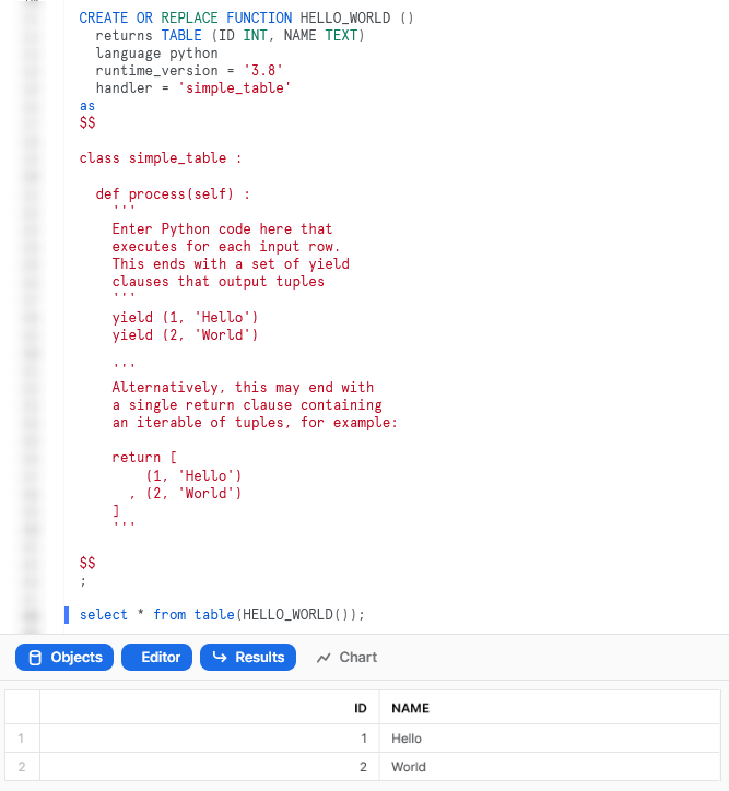
Return a Simple Table

Our first example is a very simple function that returns a static table. First, let’s see the code:

CREATE OR REPLACE FUNCTION HELLO_WORLD ()
  returns TABLE (ID INT, NAME TEXT)
  language python
  runtime_version = '3.8'
  handler = 'simple_table'
as
$$

class simple_table :
  
  def process(self) :
    '''
    Enter Python code here that 
    executes for each input row.
    This ends with a set of yield
    clauses that output tuples
    '''
    yield (1, 'Hello')
    yield (2, 'World')
    
    '''
    Alternatively, this may end with
    a single return clause containing
    an iterable of tuples, for example:
    
    return [
        (1, 'Hello')
      , (2, 'World')
    ]
    '''
    
$$
;

There are a few things to break down here to confirm our understanding:

• Starting on row 9, we have defined a very simple class in Python which acts as our handler. The class only leverages the process method, without using any inputs, and simply returns two tuples of data.
• The name of our handler class on row 5 matches that of our Python class defined on row 9.
• On row 2, we can see that our function will return a table consisting of an ID integer field and a NAME text field.

If we execute this code in a Snowflake worksheet, we can then call the table function to see the result.

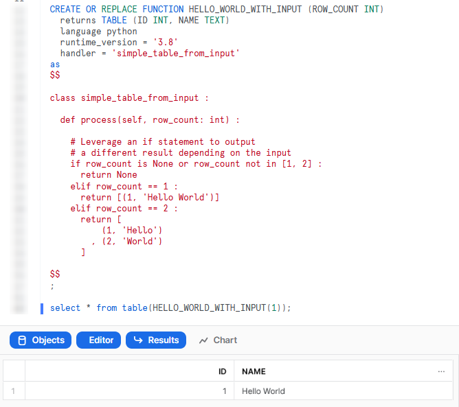
Return a Simple Table Based on an Input

Our second example is a step up from the first, following a similar process but using an input variable to determine the output. Let’s see the code:

CREATE OR REPLACE FUNCTION HELLO_WORLD_WITH_INPUT (ROW_COUNT INT)
  returns TABLE (ID INT, NAME TEXT)
  language python
  runtime_version = '3.8'
  handler = 'simple_table_from_input'
as
$$

class simple_table_from_input :
  
  def process(self, row_count: int) :

    # Leverage an if statement to output
    # a different result depending on the input
    if row_count is None or row_count not in [1, 2] :
      return None
    elif row_count == 1 :
      return [(1, 'Hello World')]
    elif row_count == 2 :
      return [
          (1, 'Hello')
        , (2, 'World')
      ]
    
$$
;

This example steps up in difficulty from the first, introducing the following key concepts:

• On row 1, we can see an expected input for the UDTF. This input matches the arguments to the process method in the handler class on row 11.
• On rows 15-23, we leverage an if statement to determine a different result depending on the input.
• For our outputs, we leverage return instead of yield so that we can output the full set of records at once.
• Importantly, note that each potential output still matches the same table structure consisting of an ID integer field and a NAME text field.

Again, if we execute this code in a Snowflake worksheet, we can then call the table function to see the result.

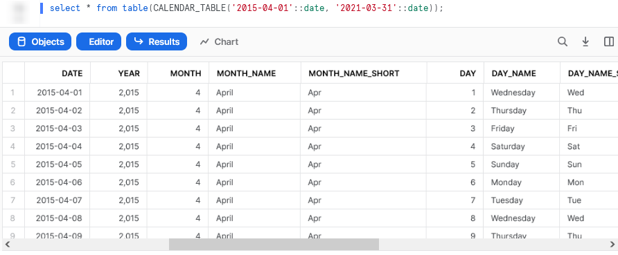
Calendar Table

The last of our simple examples takes things one step further, so that we can introduce an additional Python function in our script and demonstrate the power of list comprehension. This UDTF leverages two input dates and generates a calendar table.

Let’s see the code:

CREATE OR REPLACE FUNCTION CALENDAR_TABLE (
      START_DATE DATE
    , END_DATE DATE
  )
  returns TABLE (
        DATE DATE
      , YEAR INT
      , MONTH INT
      , MONTH_NAME TEXT
      , MONTH_NAME_SHORT TEXT
      , DAY INT
      , DAY_NAME TEXT
      , DAY_NAME_SHORT TEXT
      , DAY_OF_WEEK INT
      , DAY_OF_YEAR INT
      , WEEK_OF_YEAR INT
      , ISO_YEAR INT
      , ISO_WEEK INT
      , ISO_DAY INT
    )
  language python
  runtime_version = '3.8'
  handler = 'calendar_table'
as
$$

# Import required standard library
from datetime import date, timedelta

class calendar_table :
  
  def process(
        self
      , start_date: date
      , end_date: date
    ) :

    # Leverage list comprehension to generate dates between start and end
    list_of_dates = [start_date+timedelta(days=x) for x in range((end_date-start_date).days + 1)]

    # Leverage list comprehension to create tuples of desired date details from list of dates
    list_of_date_tuples = [
        (
            date
          , date.year
          , date.month
          , date.strftime("%B")
          , date.strftime("%b")
          , date.day
          , date.strftime("%A")
          , date.strftime("%a")
          , date.strftime("%w")
          , date.strftime("%j")
          , date.strftime("%W")
          , date.strftime("%G")
          , date.strftime("%V")
          , date.strftime("%u")
        ) 
        for date in list_of_dates
      ]

    return list_of_date_tuples
    
$$
;

This example steps up in difficulty in several ways, introducing the following key concepts:

• On rows 2-3, we can see two expected inputs for the UDTF. These inputs match the arguments to the process method in the handler class on rows 34-35, and denote the start and end dates for the returned calendar table.
• On rows 5-20, we can see that the metadata for the returned table contains several fields, including the date, year, month and day.
• On row 28, we import our required functionality from the standard Python library. As this is from the standard Python library, no further imports or configurations are required.
• On row 39, we leverage list comprehension to generate a list of dates between the provided start and end dates
• On rows 42-60, we again leverage list comprehension to create a list of tuples that contain the desired details for each date in the list of dates.
• On row 62, we leverage return instead of yield so that we can output the full set of records at once. It is critical that the output being returned is an iterable of tuples.

Again, if we execute this code in a Snowflake worksheet, we can then call the table function to see the result. This screenshot omits the code itself for brevity.

Examples Leveraging Partitioned Data

Now that we have some simple examples under our belt, it’s time to progress to some examples leveraging input data. In my opinion, this is where UDTFs really start to shine and demonstrate their potential.

Running Sum

This is a simple example that demonstrates using partitioning within a UDTF to act on a tabular input. Of course, we could easily achieve the same result using a standard window function in SQL, but we are trying to demonstrate functionality here and this is a simple example.

Let’s see the code:

CREATE OR REPLACE FUNCTION GENERATE_RUNNING_SUM (
      INPUT_MEASURE FLOAT
  )
  returns TABLE (
      RUNNING_SUM FLOAT
    )
  language python
  runtime_version = '3.8'
  handler = 'generate_running_sum'
as
$$

# Define handler class
class generate_running_sum :

  ## Define __init__ method that acts
  ## on full partition before rows are processed
  def __init__(self) :
    # Create initial running sum variable at zero
    self._running_sum = 0
  
  ## Define process method that acts
  ## on each individual input row
  def process(
        self
      , input_measure: float
    ) :

    # Increment running sum with data
    # from the input row
    new_running_sum = self._running_sum + input_measure
    self._running_sum = new_running_sum

    yield(new_running_sum,)
  
$$
;

The core difference between this UDTF and our previous examples are:

• On rows 18-20, we have now included the __init__ method within our class. We use this method to declare a variable called _running_sum within self that begins with zero value.
• On row 31, we leverage the self._running_sum variable to calculate the new running sum for the current row. If this is the first row, the self._running_sum value will be zero as we initialised on row 20. If this is not the first row, it will use the previous row’s final value of self._running_sum which we set on row 32.
• It would be tempting to yield self._running_sum itself on row 34 instead of an interim variable such as new_running_sum; however, this would be reading the value from the original input instead of the updated value, and thus would not include any of the change we make. If you attempt this yourself, you will find it returns the same as the input instead of a running total.
• Our yield statement on row 34 looks slightly strange due to the comma near the end. We must leverage this comma to ensure that our single-value output is treated as a tuple instead of a scalar variable.

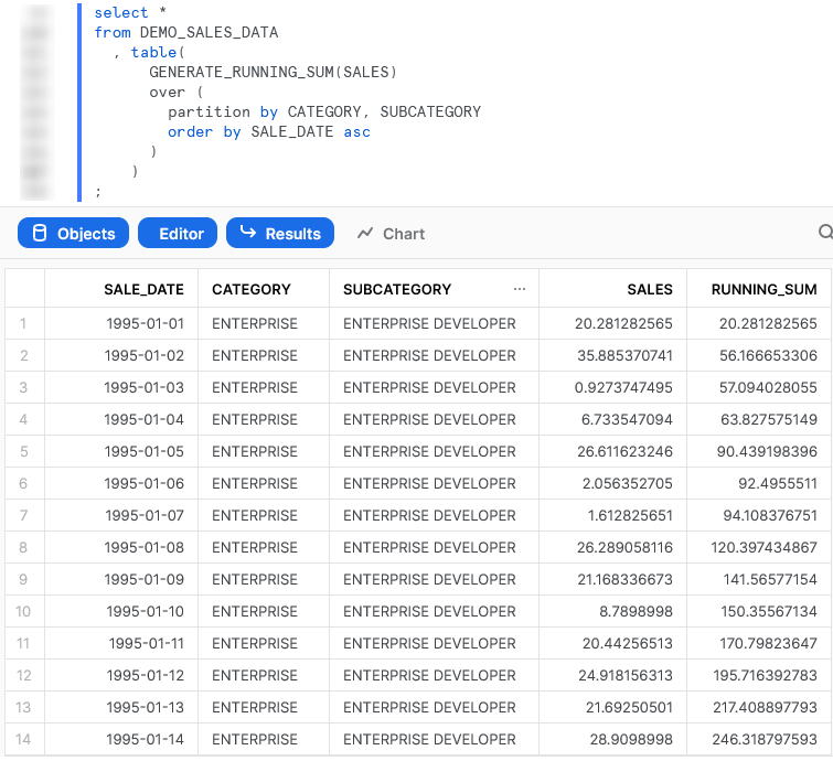
When calling the UDTF using values from another query as an input, we leverage the following SQL statement. This statement queries a table called DEMO_SALES_DATA and uses comma notation to indicate leveraging a tabular UDTF. This is similar to when performing a lateral flatten to parse semi-structured data. We must also strictly determine which fields we wish to partition our data by and the order in which rows should be submitted, similar to how we would for a window function.

select * 
from DEMO_SALES_DATA
  , table(
      GENERATE_RUNNING_SUM(SALES) 
      over (
        partition by CATEGORY, SUBCATEGORY
        order by SALE_DATE asc
      )
    )
;

Again, if we execute this code in a Snowflake worksheet, we can then call the table function to see the result. This screenshot omits the UDTF code itself for brevity.

Average

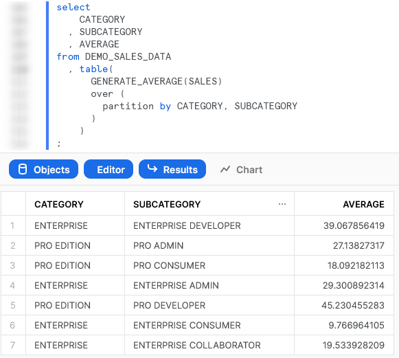
Our next example again takes things one step further, but is not an efficient or particular useful UDTF. We purely include this to demonstrate the functionality before diving into our more complex examples below. In this example, we read in all of the values for the partition first, then use those values to return the average value for each partition. This would be easily achieved using a simple GROUP BY function in SQL paired with the AVG function.

Let’s see the code:

CREATE OR REPLACE FUNCTION GENERATE_AVERAGE (
      INPUT_MEASURE FLOAT
  )
  returns TABLE (
      AVERAGE FLOAT
    )
  language python
  runtime_version = '3.8'
  handler = 'generate_average'
as
$$

# Define handler class
class generate_average :

  ## Define __init__ method that acts
  ## on full partition before rows are processed
  def __init__(self) :
    # Create initial empty list to store values
    self._values = []
  
  ## Define process method that acts
  ## on each individual input row
  def process(
        self
      , input_measure: float
    ) :

    # Increment running sum with data
    # from the input row
    self._values.append(input_measure)

  ## Define end_partition method that acts
  ## on full partition after rows are processed
  def end_partition(self) :
    values_list = self._values

    average = sum(values_list) / len(values_list)

    yield(average,)

$$
;

The core difference between this UDTF and our previous example is the inclusion of the end_partition method on rows 88-93 which acts on the full list of input values after they have been collected by the process method.

Again, if we execute this code in a Snowflake worksheet, we can then call the table function to see the result. This screenshot omits the code itself for brevity.

Importing Additional Libraries from Anaconda

Even though our examples so far have all been fairly basic, we can already start to see how powerful Python UDTFs could be. Not only are we able to receive inputs and use them to produce outputs, we can also define our own functionality within the Python script and perform more complex logical steps when executing our function.

What about if we wish to use Python libraries that are not part of the standard inbuilt set? For example, what if we wish to leverage Pandas, PyTorch, or a wide range of other popular libaries? The good news here is that Snowflake have partnered with Anaconda and you already have everything you need to leverage any of the libraries listed in Anaconda’s Snowflake channel.

If you wish to leverage any libraries that are not included in Anaconda’s Snowflake channel, including any libraries you have developed in-house, then you will need to import them separately. This will be discussed in the next section.

Accepting the Terms of Usage to Enable Third-Party Packages

To leverage third party packages from Anaconda within Snowflake, an ORGADMIN must first accept the third party terms of usage. I walk through the process now, however more details can be found here for those who desire it. This step must only be completed once for the entire organisation.

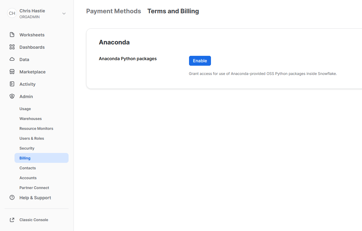
1. Using the ORGADMIN role in the SnowSight UI, navigate to Admin > Billing to accept the third party terms of usage:
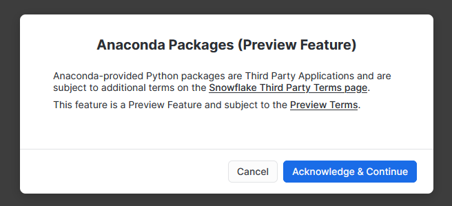
2. Confirm acknowledgement:
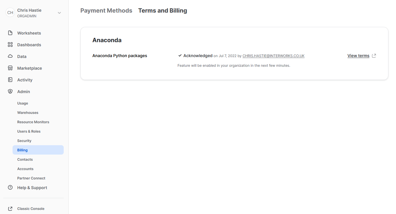
3. The screen will then update to reflect the accepted terms:

Examples Using Supported Third-Party Libraries

Now that we have enabled third-party libraries for our organisation, we can show some more interesting examples.

Train and Deploy an ARIMA Machine Learning Model

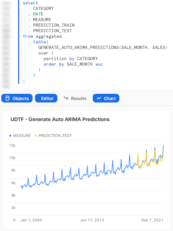
This function imports the pmdarima library to train an ARIMA model and then test it, using an 80/20 train/test split. This is useful to demonstrate some of the powerful functionality that is unlocked when you combine Python and Snowflake.

It is important to note at this time that I am not a data scientist by trade and am simply demonstrating functionality, however I am open to any feedback or knowledge about how this demonstration could be improved. You can also learn more about this approach by attending the session that Thoughtspot’s Sonny Rivera and myself are running at this year’s Snowflake BUILD 2022 Data Cloud Dev Summit.

Let’s see the code:

CREATE OR REPLACE FUNCTION GENERATE_AUTO_ARIMA_PREDICTIONS (
      INPUT_DATE DATE
    , INPUT_MEASURE FLOAT    
  )
  returns TABLE (
        DATE DATE
      , MEASURE FLOAT
      , PREDICTION_TRAIN FLOAT
      , PREDICTION_TEST FLOAT
    )
  language python
  runtime_version = '3.8'
  packages = ('pandas', 'pmdarima')
  handler = 'generate_auto_arima_predictions'
as
$$

import pandas
import pmdarima
from datetime import date

class generate_auto_arima_predictions :

  def __init__(self) :
    # Create empty list to store inputs
    self._data = []
  
  def process(
        self
      , input_date: date
      , input_measure: float
    ) :

    # Ingest rows into pandas DataFrame
    data = [input_date, input_measure]
    self._data.append(data)

  def end_partition(self) :

    # Convert inputs to DataFrame
    df_input = pandas.DataFrame(data=self._data, columns=["DATE", "MEASURE"])

    # Determine test and train splits of the data
    # leverage an 80:20 ratio.
    train_data, test_data = pmdarima.model_selection.train_test_split(df_input["MEASURE"], test_size=0.2)

    # Create Auto Arima model
    model = pmdarima.auto_arima(
          train_data
        , test='adf'
        , max_p=3, max_d=3, max_q=3
        , seasonal=True, m=12, max_P=3
        , max_D=2, max_Q=3, trace=True
        , error_action='ignore'
        , suppress_warnings=True
        , stepwise=True
      )
    
    # Convert train and test values to dataframes
    df_train = pandas.DataFrame(data=train_data, columns=["MEASURE_TRAIN"])
    df_test = pandas.DataFrame(data=test_data, columns=["MEASURE_TEST"])

    # Generate in-sample predictions
    pred_train = model.predict_in_sample(dynamic=False) # works only with auto-arima
    df_train = pandas.DataFrame(
        data=pandas.to_numeric(pred_train)
      , columns=["PREDICTION_TRAIN"]
    )

    # Generate predictions on test data
    pred_test = model.predict(n_periods=len(test_data), dynamic=False)
    df_test = pandas.DataFrame(
        data=pandas.to_numeric(pred_test)
      , columns=["PREDICTION_TEST"]
    )
    # Adjust test index to align with
    # the end of the training data
    df_test.index += len(df_train)

    # Combine test and train prediction values with original
    df_output = pandas.concat([df_input, df_train, df_test], axis = 1) \
      [["DATE", "MEASURE", "PREDICTION_TRAIN", "PREDICTION_TEST"]]
                              
    # Output the result
    return list(df_output.itertuples(index=False, name=None))

    '''
    Alternatively, the output could be returned
    by iterating through the rows and yielding them
    for index, row in df_output.iterrows() :
      yield(row[0], row[1], row[2], row[3])
    '''

$$
;

The core difference between this UDTF and our previous examples are:

• On row 13, we have now included a line to include the pandas and pmdarima libraries in the metadata for the UDTF.
• On rows 18-19, we import the pandas and pmdarima libraries for use in our Python code.

Again, if we execute this code in a Snowflake worksheet, we can then call the function whilst specifying our desired partitions to see the result. Here we display the chart from Snowsight instead of the tabular output so that we can clearly demonstrate how our test predictions compare with our original values.

Train and Deploy a scikit Learn Linear Regression Model

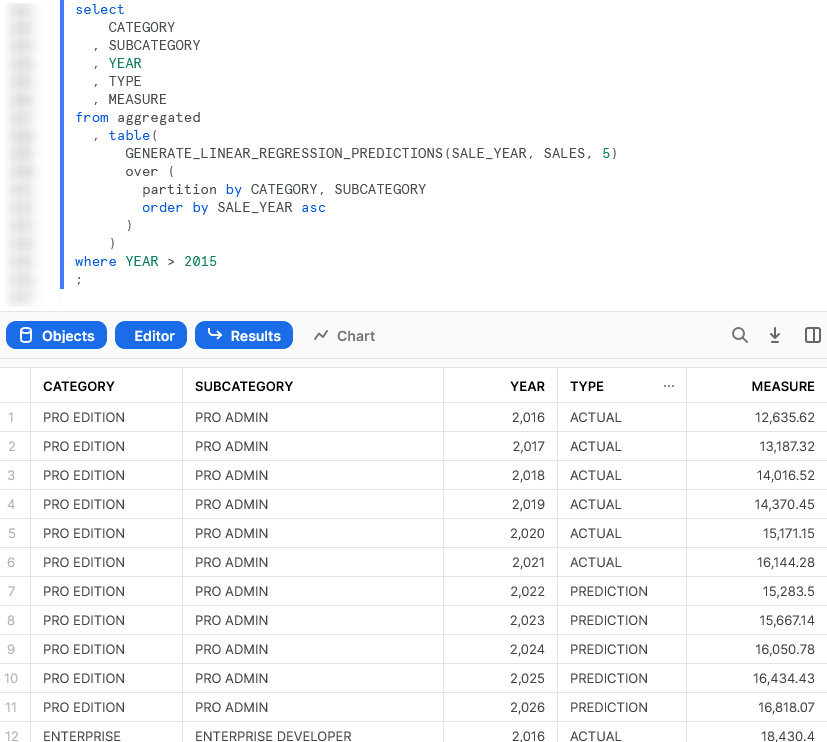
This function imports the scikit learn library to train a linear regression model and then use it to generate a handful of predicted values.

Again, it is important to note at this time that I am not a data scientist by trade and am simply demonstrating functionality; however, I am open to any feedback or knowledge about how this demonstration could be improved.

Let’s see the code:

CREATE OR REPLACE FUNCTION GENERATE_LINEAR_REGRESSION_PREDICTIONS (
      INPUT_YEAR INT
    , INPUT_MEASURE FLOAT
    , INPUT_PERIODS_TO_FORECAST INT  
  )
  returns TABLE (
        YEAR INT
      , TYPE TEXT
      , MEASURE FLOAT
    )
  language python
  runtime_version = '3.8'
  packages = ('pandas', 'scikit-learn')
  handler = 'generate_linear_regression_predictions'
as
$$

# Import modules
import pandas
from sklearn.linear_model import LinearRegression
from datetime import date

# Define handler class
class generate_linear_regression_predictions :

  ## Define __init__ method that acts
  ## on full partition before rows are processed
  def __init__(self) :
    # Create empty list to store inputs
    self._data = []
  
  ## Define process method that acts
  ## on each individual input row
  def process(
        self
      , input_year: date
      , input_measure: float
      , input_periods_to_forecast: int
    ) :

    # Ingest rows into pandas DataFrame
    data = [input_year, 'ACTUAL', input_measure]
    self._data.append(data)
    self._periods_to_forecast = input_periods_to_forecast

  ## Define end_partition method that acts
  ## on full partition after rows are processed
  def end_partition(self) :

    # Convert inputs to DataFrame
    df_input = pandas.DataFrame(data=self._data, columns=["YEAR", "TYPE", "MEASURE"])

    # Determine inputs for linear regression model
    # x = pandas.DatetimeIndex(df_input["DATE"]).year.to_numpy().reshape(-1, 1)
    x = df_input["YEAR"].to_numpy().reshape(-1, 1)
    y = df_input["MEASURE"].to_numpy()

    # Create linear regression model
    model = LinearRegression().fit(x, y)

    # Determine forecast range
    periods_to_forecast = self._periods_to_forecast
    # Leverage list comprehension to generate desired years
    list_of_years_to_predict = [df_input["YEAR"].iloc[-1] + x + 1 for x in range(periods_to_forecast)]
    
    prediction_input = [[x] for x in list_of_years_to_predict]
    
    # Generate predictions and create a df
    predicted_values = model.predict(prediction_input)
    predicted_values_formatted = pandas.to_numeric(predicted_values).round(2).astype(float)
    df_predictions = pandas.DataFrame(
        data=predicted_values_formatted
      , columns=["MEASURE"]
    )

    # Create df for prediction year
    df_prediction_years = pandas.DataFrame(
        data=list_of_years_to_predict
      , columns=["YEAR"]
    )

    # Create df for prediction type
    prediction_type_list = ["PREDICTION" for x in list_of_years_to_predict]
    df_prediction_type = pandas.DataFrame(
        data=prediction_type_list
      , columns=["TYPE"]
    )

    # Combine predicted dfs into single df
    df_predictions_combined = pandas.concat([df_prediction_years, df_prediction_type, df_predictions], axis = 1) \
      [["YEAR", "TYPE", "MEASURE"]]

    # Adjust test index to align with
    # the end of the training data
    df_predictions.index += len(df_input)

    # Combine predicted values with original
    df_output = pandas.concat([df_input, df_predictions_combined], axis = 0) \
      [["YEAR", "TYPE", "MEASURE"]]

    # Output the result
    return list(df_output.itertuples(index=False, name=None))
  
    '''
    Alternatively, the output could be returned
    by iterating through the rows and yielding them
    for index, row in df_output.iterrows() :
      yield(row[0], row[1], row[2])
    '''

$$
;

This example is very similar to the Auto ARIMA example and simply serves as another opportunity to demonstrate the functionality here.

Again, if we execute this code in a Snowflake worksheet, we can then call the function whilst specifying our desired partitions to see the result. Here we can see 5 predicted values along with the final actual values for the partition.

Importing Files and Libraries via a Stage

So far, we have demonstrated quite a lot in our miniature crash course into Python UDTFs in Snowflake. Before we wrap up, I’d like to cover one last piece, which is how to import libraries that are not covered by the Anaconda Snowflake channel and how to import other external files.

Warning Regarding Staged Files and Libraries

It is important to note at this time that these external files are fixed in time. UDTFs do not have access to the “outside world” and each file must exist within the stage at the time the UDTF is created, as the file is actually copied into Snowflake’s underlying storage location for the UDTF. If you update your files in your external stage, your Snowflake UDTF will not undergo these changes unless you recreate the UDTF as well.

Unfortunately, files must be imported into UDTFs individually and specifically. If you wish to import five files within a directory, you must list all 5 files individually. You cannot simply specify a parent directory or leverage a wildcard.

Examples Using External Files and Libraries

For these examples, we will be uploading all of our required files to the stage “STG_FILES_FOR_UDTFS.”

Import an External Excel xlsx File

This example reads an Excel xlsx file into a pandas dataframe, then uses information in that file to map the input string to the corresponding output.

The file we will be leveraging is a very simple mapping file that looks like this:

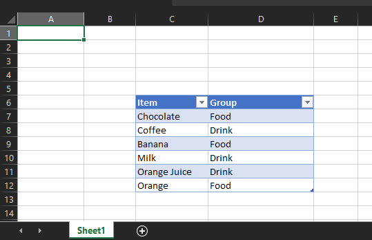
The file is called “Dummy Mapping File.xlsx,” and I have uploaded it to the stage “STG_FILES_FOR_UDTFS.”

Here is the code for the UDTF itself:

CREATE OR REPLACE FUNCTION LEVERAGE_EXTERNAL_MAPPING_FILE (
      INPUT_ITEM STRING
  )
  returns TABLE (
      MAPPED_ITEM STRING
    )
  language python
  runtime_version = '3.8'
  packages = ('pandas', 'openpyxl') -- openpyxl required for pandas to read xlsx
  imports = ('@STG_FILES_FOR_UDTFS/Dummy Mapping File.xlsx')
  handler = 'leverage_external_mapping_file'
as
$$

# Import the required modules 
import pandas
import sys

# Retrieve the Snowflake import directory
IMPORT_DIRECTORY_NAME = "snowflake_import_directory"
import_dir = sys._xoptions[IMPORT_DIRECTORY_NAME]

# Ingest the mapping into a Pandas dataframe
df_mapping = pandas.read_excel(import_dir + 'Dummy Mapping File.xlsx', skiprows=5, usecols="C:D")

# Define handler class
class leverage_external_mapping_file :
  
  ## Define process method that acts
  ## on each individual input row
  def process(
        self
      , input_item: str
    ) :

    ### Apply the mapping to retrieve the mapped value
    df_mapped_group = df_mapping[df_mapping['Item']==input_item]
  
    mapped_group = 'No matching group found'
    
    if len(df_mapped_group.index) > 0 :
      mapped_group = df_mapped_group.iloc[0]['Group']

    yield(mapped_group,)
  
$$
;

The unique differences for this example are:

• Row 10 includes a line to import the file from a stage. This is a critical component for our Python function to be able to access the file during the pandas.from_excel() method.
• Mirroring this is the code on lines 20-21 that leverages the sys library to access the location where Snowflake stores files that have been imported into the UDTF. The file is then ingested using pandas on row 24.

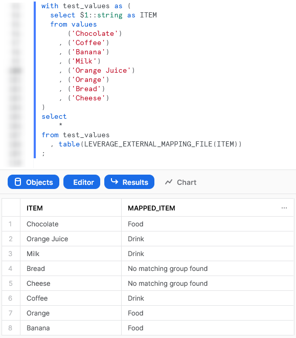
The rest of the code in this script is specific Python code to download the Excel file into a dataframe, filter it to our specific item and return the matched group value.

Again, if we execute this code in a Snowflake worksheet, we can then call the function to see the result.

Import a Non-Standard External Library

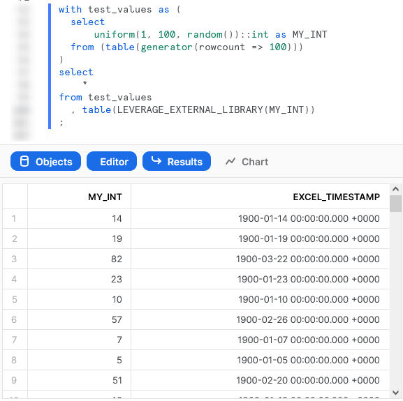
This example is designed to leverage the xldate function of the xlrd library. This library is not included in the standard set of supported libraries,  so it must be imported specifically.

Let’s see the code:

CREATE OR REPLACE FUNCTION LEVERAGE_EXTERNAL_LIBRARY (
      INPUT_INT INTEGER
  )
  returns TABLE (
      EXCEL_TIMESTAMP TIMESTAMP
    )
  language python
  runtime_version = '3.8'
  imports = ('@STG_FILES_FOR_UDTFS/xlrd/xldate.py')
  handler = 'leverage_external_library'
as
$$

# Import the required modules 
import sys

# Retrieve the Snowflake import directory
IMPORT_DIRECTORY_NAME = "snowflake_import_directory"
import_dir = sys._xoptions[IMPORT_DIRECTORY_NAME]

# Import the required external modules using the importlib.util library
import importlib.util
module_spec = importlib.util.spec_from_file_location('xldate', import_dir + 'xldate.py')
xldate = importlib.util.module_from_spec(module_spec)
module_spec.loader.exec_module(xldate)

# Define handler class
class leverage_external_library :
  
  ## Define process method that acts
  ## on each individual input row
  def process(
        self
      , input_int: int
    ) :

    ### Apply the mapping to retrieve the mapped value
    xl_datetime = xldate.xldate_as_datetime(input_int, 0)

    yield(xl_datetime,)
  
$$
;

The unique differences for this example are:

• Row 9 includes a line to import the xldate.py file from a stage. This is critical, and would match the file found in your env/Lib/site-packages/xlrd directory that is created during a pip install in a virtual environment (or your default environment).
• As with the previous example, lines 18-19 leverage the sys library to access the location where Snowflake stores files that have been imported into the UDTF.
• The block of lines 22-25 leverage the importlib.util library to import the specific module from the imported directory. This imported library is then leveraged on row 38.

Again, if we execute this code in a Snowflake worksheet, we can then call the function to see the result. In this example, the test values are created using Snowflake’s generator function.

Wrap Up

So there we have it. We have covered a lot of content in this post and some of these UDTFs could potentially have their own blog post all on their own! My goal is to demonstrate how to create UDTFs for different scenarios and provide that in a single post so that it is easy for readers to find and refer back to if needed.

I hope this helps you get started on your own journey with Python UDTFs in Snowflake. Let us know what cool things you come up, it’s always great to see new functionality lead to productive and useful innovation.

If you wish to see the code for all of this and other content that we have, you can find it on the InterWorks GitHub.

If you are interested in finding out about Python UDFs or stored procedures instead of UDTFs, or wish to achieve this with Snowpark instead of through the UI, be sure to check out my other Definitive Guides for Snowflake with Python.