This series shows you the various ways you can use Python within Snowflake.

Recently, I was involved in a project which required using geospatial (basically maps) data for an analytical application. Now, with ESRI shape files being around for more than three decades, any sincere BI application like Tableau can easily read and work with these spatial files. But Snowflake has geospatial data types available, too; and when there is a need to combine the geospatial data with other data or to process it in a performant manner, Snowflake has the edge rather than storing and referring these files locally. Besides, recently Snowflake has made reading files dynamically in a Python Snowpark function possible. Daria Rostovtseva from Snowflake has written a crisp article about loading shape file archives using Python Snowpark UDTF. So, I thought I would make use of it right away and make life (and analysis) simpler. Little did I know that I had embarked on a small adventure.

Loading the Shape Data

As the project required UK geographical data, my colleague Max provided me with some excellent publicly available datasets from 2011 UK census. Following the above article, it is fairly straightforward to load the data. The entire shape file ZIP archive is required to decipher the data and not just the .shp file. Simply create an internal stage, load the shape data archive there and then use the Snowpark Python table function py_load_geofile given in blog to load the data into a table.

create int_stage;
put file://infuse_dist_lyr_2011.zip @int_stage/shape_files parallel = 8 auto_compress = false source_compression = auto_detect;

create or replace table local_area_districts_staged as
select 
    properties,
    to_geography(wkb, True) as geo_features
from table(
    py_load_geofile(
        build_scoped_file_url(@int_stage, 'shape_files/infuse_dist_lyr_2011.zip')
                                        , 'infuse_dist_lyr_2011.shp'
    )
);

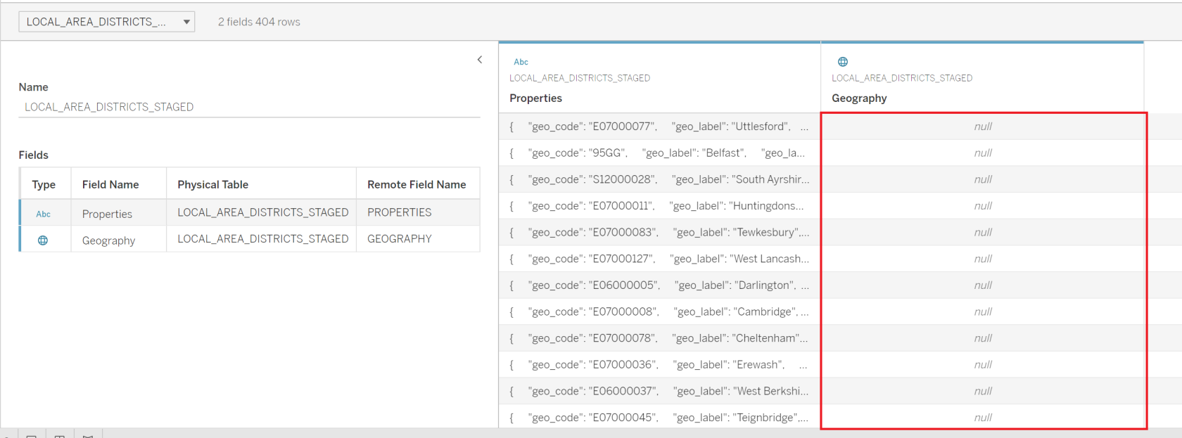
It loaded uneventfully; but when referred in Tableau, Tableau didn’t like it, although the data types were what they should have been.

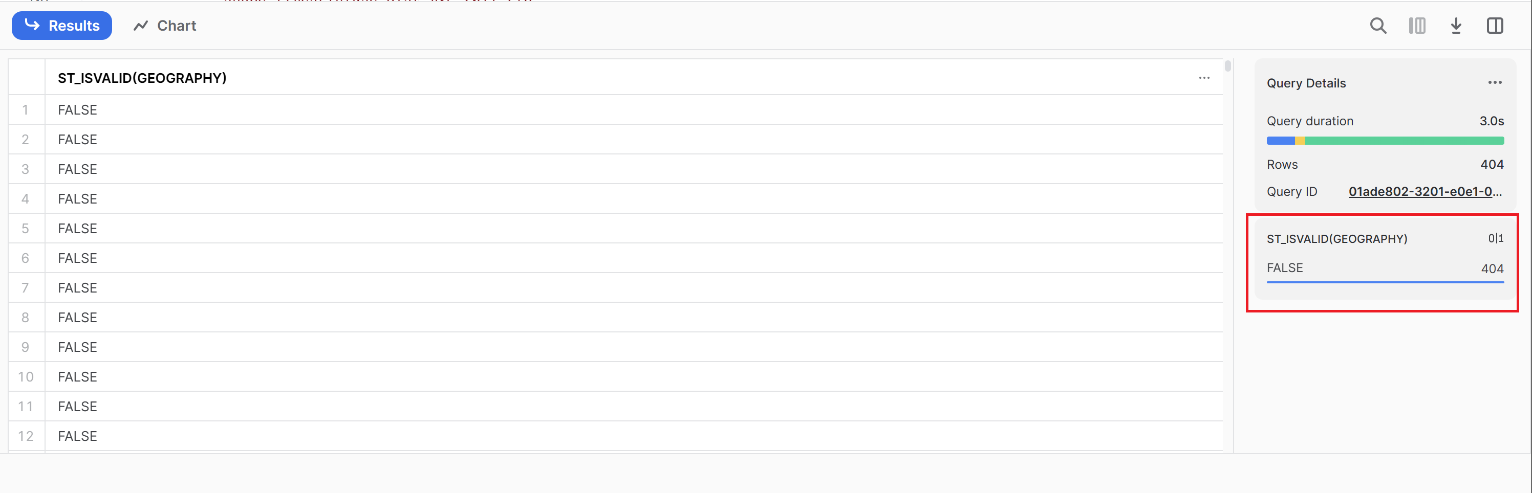
The first suspect for a data engineer is always the data. Snowflake provides a neat function, st_isvalid, to check whether the underlying geographical data is valid or not.

select st_isvalid(geography)
from local_area_districts_staged;

To my shock, every value in the geography column was invalid!

But in this case, data couldn’t be doubted as it was officially published governmental data. It left me thinking, and when I started looking for clues, I came across this statement in Daria’s blog which I had overlooked before:

It’s important to be aware of the shapefile’s spatial reference. If geographic coordinates are unprojected (i.e., representing locations on the Earth’s surface as points on a 3D sphere using WGS84 geographic coordinate system), it is appropriate to parse the geographic coordinates into Snowflake’s geography data type. In my example, the data is in WGS84, and parsed using to_geography function. If the coordinates are projected (representing locations on the Earth’s surface using a two-dimensional Cartesian coordinate system), they should be parsed into geometry data type using one of the geometry functions. To figure out if the shapefile is projected or unprojected, you can look at the .prj file inside the zipped shapefile archive.

The CTAS statement to import the data was thus updated to load a column of type geometry instead of geography as follows.

create or replace table local_area_districts_staged as
select 
    properties,
    to_geometry(wkb, False) as geo_features
from table(
    py_load_geofile(
        build_scoped_file_url(@int_stage, 'shape_files/infuse_dist_lyr_2011.zip')
                                        , 'infuse_dist_lyr_2011.shp'
    )
);

Please note the call to the to_geometry function. The value of the second parameter, <allow_invalid>, had now been set to False to perform stricter loading and to reject invalid shapes. Keen readers would notice that in the first version of the CTAS statement (see above), this parameter value to to_geography function was True, which is why Snowflake accepted the invalid geographical coordinates in first place. However, this was far from a solution as Tableau would still require the geographical coordinates in longitude/latitude format.

Finding and Converting the Coordinate Encoding

My knowledge about geospatial data and systems being less than elementary, that was a real puzzle for me now. But a close look at some data points (for example, (291902, 196289)) told me that these are not longitude/latitude data! WSG84 meant longitude/latitude data. Now a word (or a paragraph rather!) on geographical coordinate systems is necessary here. WGS or World Geodetic System is a “standard used in cartography, geodesy and satellite navigation including GPS,” according to Wikipedia, and 84 is the current version of the standard so the longitude/latitude numbers in layman’s terms become WGS84 encoded coordinates. The .prj file in the data archive had some really cryptic information out of which following seemed interesting. “OSGB_1936_British_National_Grid.“

Using a Built-in Snowflake Function

Fortunately, Snowflake has recently released a st_transform function into GA. With this function, it is easy to convert the spatial reference system of any coordinates into any other system. When the “from” and “to” SRID of the coordinate systems are known, the conversion is simply a function call on the column which contains the geospatial data.

ST_TRANSFORM( <geometry_expression> [ , <from_srid> ] , <to_srid> );

A simple search for the SRIDs for OSGB_1936_British_National_Grid and WGS84 showed that their SRIDs are 27700 and 4326 respectively (WGS84 has many coordinate systems, but one that is relevant to it, is 4326, as per the Snowflake documentation.). That means the conversion could be simply:

select st_transform(geometry, 27700, 4326) from local_area_districts_staged

But there is one things to keep in mind. The st_transform function returns GEOMETRY data type and not GEOGRAPHY data type. So the final table creation statement became,

create or replace table local_area_districts
as
select properties, try_to_geography(st_aswkb(st_transform(geometry, 27700, 4326))) as geography
from local_area_districts_staged;

A quick test with Tableau showed that Tableau was happy about this data and could read it as geospatial map data (screenshot similar to one in the end of this post).

Now, this could very well be the end of this post as the goal was achieved, but something was still on my mind: The .prj file that came with the data, which I previously mentioned, had much more descriptive content. Following to be precise.

PROJCS[
  "OSGB_1936_British_National_Grid",
  GEOGCS["GCS_OSGB 1936",
    DATUM[
      "D_OSGB_1936",
      SPHEROID["Airy_1830",6377563.396,299.3249646]
    ],
    PRIMEM["Greenwich",0],
    UNIT["Degree",0.017453292519943295]
  ],
  PROJECTION["Transverse_Mercator"],
  PARAMETER["latitude_of_origin",49],
  PARAMETER["central_meridian",-2],
  PARAMETER["scale_factor",0.9996012717],
  PARAMETER["false_easting",400000],
  PARAMETER["false_northing",-100000],
  UNIT["Meter",1]
]

There was a lot of information there for which the st_transform function had no regard. In all fairness, it did solve my purpose, but what if all this extra information is required to achieve projection or conversion accuracy? How to use this information as there is no way to provide this information to st_transform function. That time it clicked me, Python has solution for everything! If I could find a pythonic way of coordinate conversion, could Snowpark help me?

Using Snowpark Python UDF to Convert Coordinates

pyproj Transformer

The brainwave I got was not going to make me a geoinformatics expert in one day, but thankfully these days we have a very powerful assistance available. I sought help of ChatGPT.

The biggest help from ChatGPT was determining which Python package to use and the boilerplate code. Credit should be given where it is due, but although it was a great help to set me on the right course, it was by no means a simple copy and paste work. A lot more needed to be done in order to upgrade this code into “production” grade code. It’s also worth noting that British Geological Survey provides a webservice as well as a detailed SQL process for bulk conversion of coordinates. Both of which were unsuitable for this use case due to various factors like dependencies and scale. A native Python Snowpark UDF was better choice and the crux of this new solution therefore remained the conversion function convert_bng_to_latlon provided (and so beautifully drafted) by ChatGPT.

The transformer.transform function suggested by ChatGPT has been deprecated since 2.6.1. version of pyproj library. The newest version (3.6.0 as of writing this article) has class named Transformer, which is recommended for all these conversion tasks. There are multiple ways to create object of Transformer class. One can simply specify the EPSG string or create a pyproj.crs.CRS object from elaborate  settings like given above.

That means, however, the following code is sufficient and would work:

from pyproj import Transformer

transformer = Transformer.from_crs(
  "EPSG:27700" # British National Grid (OSGB)
  , "EPSG:4326" # WGS84 (latitude and longitude)
)

This next way of creating a Transformer object is much better way to preserve all the characteristics of the source CRS:

from pyproj import Transformer, CRS

crs_str = '''
PROJCS[
  "OSGB_1936_British_National_Grid"
  ,GEOGCS[
    "GCS_OSGB 1936"
    ,DATUM[
      "D_OSGB_1936"
      ,SPHEROID["Airy_1830",6377563.396,299.3249646]
    ]
    ,PRIMEM["Greenwich",0]
    ,UNIT["Degree",0.017453292519943295]
  ]
  ,PROJECTION["Transverse_Mercator"]
  ,PARAMETER["latitude_of_origin",49]
  ,PARAMETER["central_meridian",-2]
  ,PARAMETER["scale_factor",0.9996012717]
  ,PARAMETER["false_easting",400000]
  ,PARAMETER["false_northing",-100000]
  ,UNIT["Meter",1]
]
'''

# Create an explicit CRS object
in_crs = CRS(crs_str)
# Define the coordinate systems
transformer = Transformer.from_crs(
  crs_from=in_crs
  , crs_to='EPSG:4326'
  , always_xy=True
)

There is a plethora of other parameters which the from_crs function accepts, which are explained well in the pyproj Transformer documentation.

Snowflake requires the geographic data in longitude and latitude format and not in latitude/longitude format as the Transformer.transform function would normally provide. The always_xy parameter takes care of swapping the result values in x and y format.

Maintaining the Structure of the Shape Data

The geospatial objects in any format (WKT, WKB, GeoJSON, etc.) are collection of coordinate values for various shapes. The actual nature of the shape would determine how many coordinates are required and even further rules can be applicable. For example, a Point shape would only require a pair of coordinates, whereas a LineString shape would require two (or more) coordinate pairs. Shapes like Polygon and MultiPolygon not only require several pairs of coordinates, they also require the first and last coordinate to nicely complete the shape and preferably no overlaps in the edges that the resultant shape would form.

The data in question contained mostly Polygons and MultiPolygons, which are represented as lists or multi-lists of tuples. For MultiPolygons, there is one more nesting of lists. This structure of the data must be kept intact while converting the values to maintain the validity of the shape. In the example below, notice one more level of nesting for the type MultiPolygon. See what all things the built in function st_transform does for us!

{
  "coordinates": [
    [
      [
        5.319848470000000e+05,
        1.818774940000000e+05
      ],
      [
        5.319886580000001e+05,
        1.818791160000000e+05
      ],
      ...
   ]
  ],
  "type": "Polygon"
}

{
  "coordinates": [
    [
      [
        [
          2.402629060000000e+05,
          1.271040940000000e+05
        ],
        [
          2.402652040000000e+05,
          1.271073980000000e+05
        ],
        ...
      ]
    ]
  ],
  "type": "MultiPolygon"
}

Next thing to consider was what data type a Python UDF can accept. As per SQL-Python data type mapping given in Snowflake documentation, a Python UDF can natively accept GEOGRAPHY data type as a parameter but not GEOMETRY parameter. Which meant a conversion of the column geo_features of table local_area_districts_staged to GeoJSON format was necessary before sending it to the Python UDF.

Python UDF for Geospatial Coordinate Conversion

Considering all the above points, the code for the final conversion Python UDF looked as follows:

create or replace function py_convert_to_wgs84(FROM_CRS string, GEOJSON object)
returns object
language python
runtime_version = '3.10'
packages = ('pyproj')
handler = 'convert_coordinates_to_lonlat'
as
$$
from pyproj import Transformer, CRS

def convert_coordinates_to_lonlat(FROM_CRS, GEOJSON):
  # Define the input CRS
  in_crs = CRS(FROM_CRS)
  
  # Output GeoJSON object
  out_geojson = {}  
  out_geojson['type'] = GEOJSON['type']
  # Define the coordinate systems
  transformer = Transformer.from_crs(
    crs_from = in_crs # Input CRS provided as parameter
    , crs_to = "EPSG:4326" # WGS84 (latitude and longitude)
    , always_xy = True # If true, the transform method will accept as input and return as output coordinates using the traditional GIS order, that is longitude, latitude for geographic CRS and easting, northing for most projected CRS.
  )
  
  # (Multi)List to store the converted coordinates
  wgs84_coordinates = []
  for coord_list in GEOJSON['coordinates']:
    if len(coord_list) > 1: # For Polygon type coord_list is a direct list of coordinate tuples
      # Convert each BNG coordinate to longitude and latitude
      lon_lat_coords = [transformer.transform(xycoord[0], xycoord[1]) for xycoord in coord_list]
      wgs84_coordinates.append(lon_lat_coords)
    else: # For MultiPolygon type coord_list should be a list of list of coordinates
      new_coord_list = []
      for coordinates in coord_list:
        # Convert each BNG coordinate to longitude and latitude
        lon_lat_coords = [transformer.transform(xycoord[0], xycoord[1]) for xycoord in coordinates]
        new_coord_list.append(lon_lat_coords)
      wgs84_coordinates.append(new_coord_list)

  out_geojson['coordinates'] = wgs84_coordinates

  return out_geojson
$$;

Notice, how handling for Polygon and MultiPolygon types is different. As the call to this UDF would require first converting the data type of geo_features column to something that the UDF can accept, it first needed to be converted to GeoJSON and then to an OBJECT data type. It would also use try_to_geography instead of to_geography system function to avoid failures occurred due to coordinate conversion. The SQL statement for that would be as follows.

create or replace table local_area_districts
as
select 
  properties
  , try_to_geography(
      py_convert_to_wgs84(
        'PROJCS["OSGB_1936_British_National_Grid",GEOGCS["GCS_OSGB 1936",DATUM["D_OSGB_1936",SPHEROID["Airy_1830",6377563.396,299.3249646]],PRIMEM["Greenwich",0],UNIT["Degree",0.017453292519943295]],PROJECTION["Transverse_Mercator"],PARAMETER["latitude_of_origin",49],PARAMETER["central_meridian",-2],PARAMETER["scale_factor",0.9996012717],PARAMETER["false_easting",400000],PARAMETER["false_northing",-100000],UNIT["Meter",1]]'
        , to_object(st_asgeojson(geo_features)))
      ) as geography
from local_area_districts_staged
;

The benefit of accepting the CRS settings as string is that one can provide a detailed specification, even a custom specification, which is not possible to provide to st_transform function. But at the same time, a simple EPSG code would also suffice. That means in my case, following code would also have achieved the same result.

create or replace table local_area_districts
as
select 
  properties
  , try_to_geography(
      py_convert_to_wgs84(
        'EPSG:27700'
        , to_object(st_asgeojson(geo_features)))
      ) as geography
from local_area_districts_staged
;

This flexibility is the power of using Python and Snowpark!

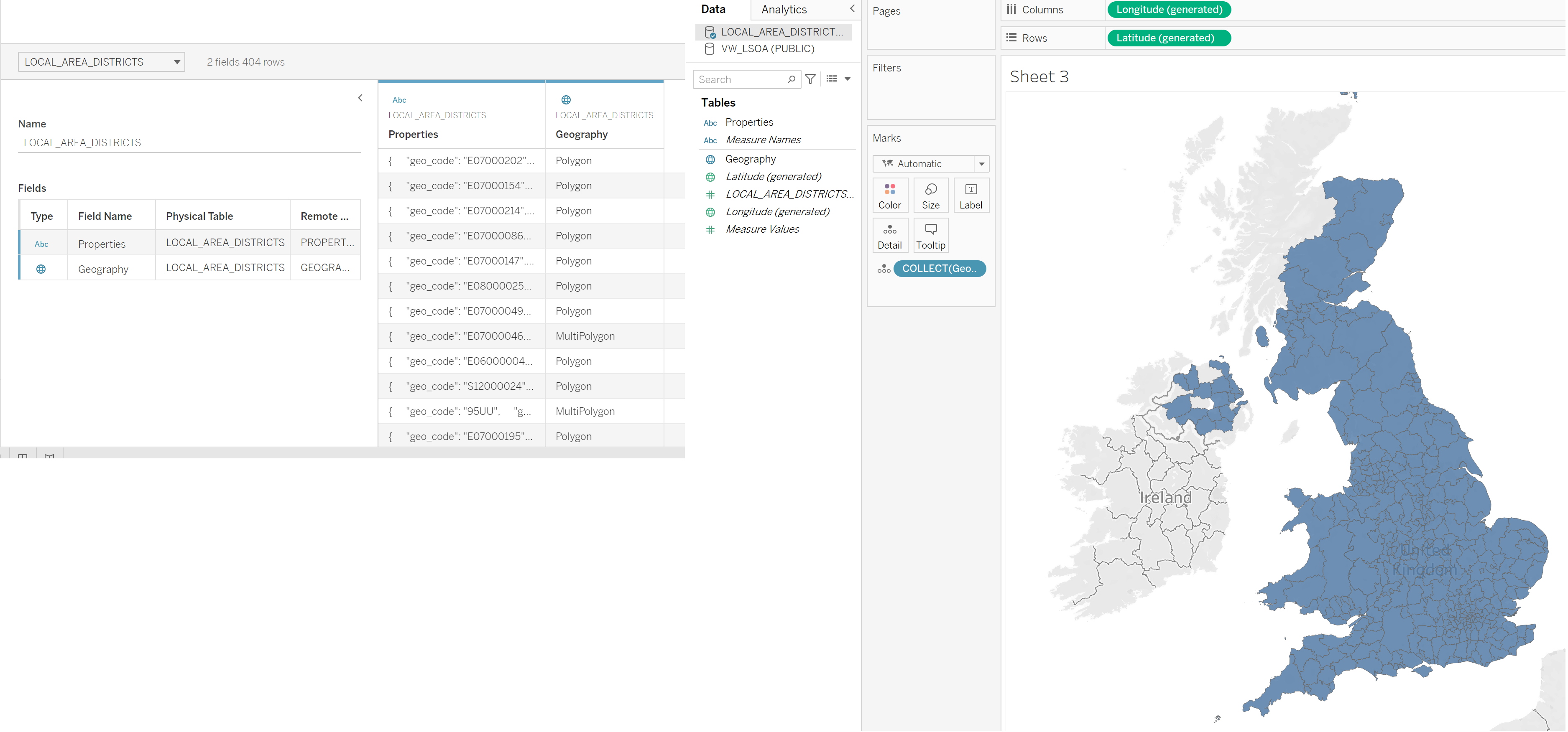
Not only Tableau recognized the shape (GEOMETRY) data created by any of the method above, but also it was able to plot it flawlessly, finally making me and my colleague Max happy.

Concluding Remarks

Snowflake is a powerful platform. Out of the box it provides a way to convert coordinates from one geospatial reference system to other. But if you want to go further than that and support custom specifications or perform some extra steps during/after conversion, you have the entire power of Python at your disposal through Snowpark. Choice is yours!

Check out the blog of my colleague, Max Giegerich, who plays with this data further to show some interesting possibilities.