
This series takes you from zero to hero with the latest and greatest cloud data warehousing platform, Snowflake.
One of Snowflake’s key selling points is automated clustering. However, it’s not immediately clear what this actually means. It’s easy to make the assumption that you will never need to think about how your data is clustered, and this is generally the case for tables under 1TB. But if you have tables larger than this (or if you’re interested in general), definitely keep reading as this may help your query performance!
Snowflake is already designed to efficiently query data and return results quickly. For larger datasets, providing a little bit of guidance to Snowflake on how to store the data can significantly reduce query times. Snowflake cannot determine this itself (how could it know which columns you are most interested in without you telling it?). However, once you have told Snowflake which fields are important, it can automatically keep your data stored in a structure that supports rapid queries using your key fields. The combination of key fields the user provides is known as the Clustering Key, but we’ll get to that.
Data Storage Architecture and Micro-Partitions
Before we talk about clustering, let’s talk about how data is stored and queried in Snowflake. To the user, Snowflake appears to store data in tables. To view data in a table, a user would simply use a query and view the results in the results pane. This is how the front-end works, but it is not how data is actually being managed and stored by Snowflake. Instead, Snowflake stores all data in encrypted files which are referred to as micro-partitions.
Each micro-partition will store a subset of the data, along with some accompanying metadata. Each micro-partition for a table will be similar in size, and from the name, you may have deduced that the micro-partition is small. Specifically, each file in Snowflake is stored in a compressed state, though if a micro-partition were to be decompressed, it would be between 50MB and 500MB in size.
The data inside each micro-partition usually spans multiple rows and columns, but this is not always the case, and it is unusual for a micro-partition to include every column in a table. Instead, micro-partitions typically span a handful of columns and rows and separate the columns within the file.
This is best explained with an example, which is supported by the following image from Snowflake’s own documentation:
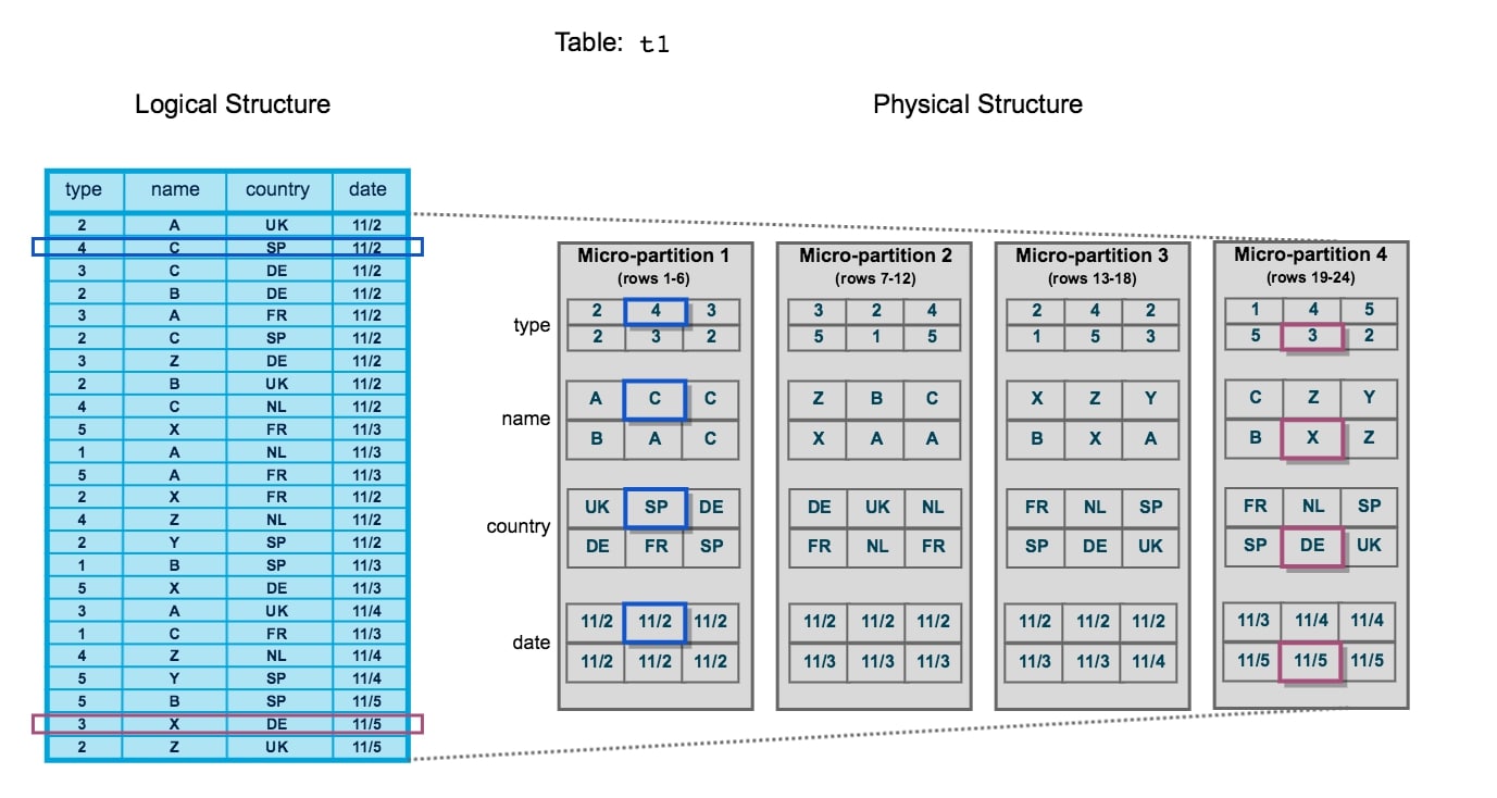
Initially, this can be a confusing diagram to take in. Let’s break it down, starting with the left-hand side. This is how a table would appear in Snowflake’s user interface or as the result of a query. This is referred to as the logical structure. We have 24 rows of data spanning four columns: type, name, country and date. Two specific rows of data have been highlighted: row 2 and row 23.
On the right-hand side is a representation of how this data would be stored in the backend of Snowflake’s architecture. This is referred to as the physical structure. Here, we can see four separate micro-partitions, each of which contains six rows of data. The first micro-partition contains data for rows 1 through 6. The data is stored by column instead of by row, enabling Snowflake to retrieve desired columns of data without breaking apart each row.
An alternative way to think about these micro-partitions is by thinking in terms of semi-structured data arrays. Recall the previous blog which introduced semi-structured data, specifically JSON structures. Whilst not the same as how Snowflake stores data, we could represent the physical structure by using four separate JSON files. For example, the first micro-partition could be represented as the following JSON array:
{
  "columns" : ["type", "name", "country", "date"],
  "rows" : [1, 2, 3, 4, 5, 6],
  "data" : [
    {
      "name": "type",
      "distinct values" : 3,
      "minimum value" : 2,
      "maximum value" : 4,
      "values" : [2, 4, 3, 2, 3, 2]
    },
    {
      "name": "name",
      "distinct values" : 3,
      "minimum value" : "A",
      "maximum value" : "C",
      "values" : ["A", "C", "C", "B", "A", "C"]
    },
    {
      "name": "country",
      "distinct values" : 4,
      "minimum value" : "DE",
      "maximum value" : "UK",
      "values" : ["UK", "SP", "DE", "DE", "FR", "SP"]
    },
    {
      "name": "date",
      "distinct values" : 1,
      "minimum value" : "11/2",
      "maximum value" : "11/2",
      "values" : ["11/2", "11/2", "11/2", "11/2", "11/2", "11/2"]
    }
  ]
}
This is a huge over-simplification of the storage method; however, this JSON representation demonstrates how some metadata is stored, as well as the values themselves.
Returning to the diagram above, rows 2 and 23 are highlighted on the left-hand side in blue and magenta, respectively. These align with the highlighted entries on the right-hand side, so we can see how these are stored in micro-partitions 1 and 4 respectively.
Query Pruning
Remember how micro-partitions store metadata in addition to the data itself? This includes important pieces of information such as which fields are within the file, the number of distinct values for each field, the range of values for each field and a few other useful pieces of information to improve performance.
This metadata is a key part of the Snowflake architecture as it allows queries to determine whether or not the data inside a micro-partition should be queried. This way, when a query is executed, it does not need to scan the entire dataset but instead only queries the micro-partitions that hold relevant data. This process is known as query pruning, as the data is pruned before the query itself is executed.
Returning to our example above, imagine a query being executed on that data to return the [type] and [country] for records where the [name] is Y:
SELECT type, country
FROM MY_TABLE
WHERE name = "Y"
;
When this query executes in Snowflake, the micro-partitions are quickly scanned to determine which contain Y as a potential entry for the [name] field. The only micro-partitions that match this criterion are micro-partitions 3 and 4. Thus, the query pruning has reduced our total dataset to just these two partitions. In a similar way, only the [type] and [country] fields are required in the query output. Any micro-partitions that do not contain data for these columns would also be pruned. When the micro-partitions themselves are queried, only the required columns are queried, and Snowflake intelligently identifies which entries match which rows and can be aligned with the original WHERE clause.
Clustering
Clustering is a common word to encounter when looking behind the scenes of a data warehouse. The idea behind clustering is to organise the storage of data to better suit expected queries. The key objectives here are to improve query performance whilst reducing the system resources required to execute queries.
For example, imagine a table with over a billion records of data across many columns. One of these columns is [category], which could be one of 10 possible values. Every day, millions of new records are added, again spanning these 10 categories.
In our example, whoever is querying this data is only ever interested in querying one or two categories at a time. With the standard method of storing data, a query with a WHERE clause that targets two categories would still query a large volume of data to return the right output. Whenever new data is added, this adds to the volume of data being queried, and there is no clean way to reduce the dataset before querying.
In Snowflake terminology, query pruning is less effective as far more micro-partitions contain multiple categories, and the desired categories in the query could easily be found in the majority of micro-partitions.
This is where clustering is effective. By restructuring how the data is stored, it is possible to improve query pruning and reduce the volume of data queried. Continuing our example, if our data was stored in a structure that was ordered by the [category] field, queries would not need to query the entire dataset. Instead, the query could skip the data up until a required [category] value appears, query the necessary records then skip the next set of records until it reaches another desired [category] value.
Let’s return to our original example demonstrated by this image:
Again, we will consider the following query:
SELECT type, country
FROM MY_TABLE
WHERE name = "Y"
;
With how the data is currently stored, this query must investigate micro-partitions 3 and 4 since both contain the value Y in the [name] field. If the intended consumer of the data often filtered the data by the [name] field, the current method of storing the data would be inefficient. Instead, we can reorganise the data into the following logical structure:
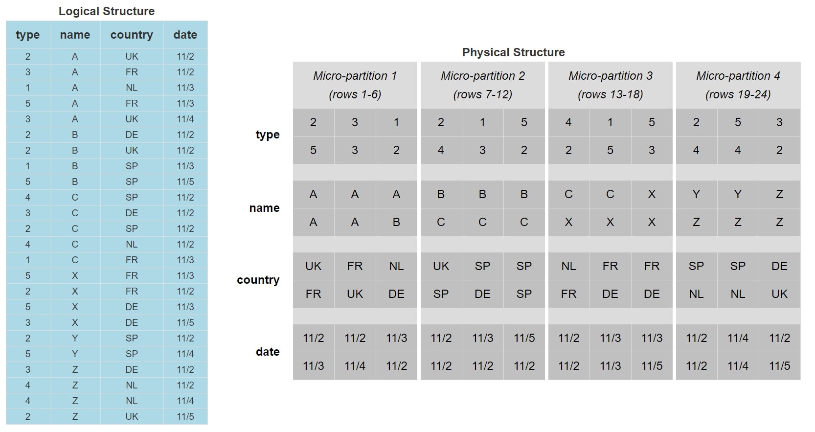
The data is now stored and ordered based on the value of the [name] field. We can see that micro-partition 4 is now the only micro-partition that contains [name] values of Y. When we execute our query now, the query pruning will reduce our target data down to just micro-partition 4, which means our query has less data to interpret and thus will perform more efficiently.
Whilst our example has dealt with a small table of only 24 rows and 4 columns, the principle behind this approach is the same as table sizes increase. Indeed, as tables increase in size, the need to cluster the data increases with it. Similarly, smaller datasets benefit from clustering far less than larger datasets, and clustering on these smaller datasets is often fruitless. Whilst being useful for demonstrating the logic behind clustering, the table we have used in our example is far too small to benefit from clustering in any recognisable way; we would expect this query to complete in under a second whether the data was clustered or not.
A General Rule to Follow
A general rule to follow when considering clustering is to consider if the table is more than 1TB in size. If so, clustering is recommended. If not, depending on how large the table is and how well queries are performing, you may consider clustering but may find it more costly than it is worth. Personally, I often test clustering by cloning the table and testing different clustering approaches on said clone. If the query performance is noticeably improved and worth the cost, I will then consider applying the clustering approach to the original table and drop the clone. A few times here I have mentioned cost, which we will revisit this further down in this post.
Clustering Keys
In the above example, we clustered our dataset based on the [Name] field, as this was a key field in our data and was used in our queries. As we have clustered based on this field, this field is referred to as the clustering key. In order to perform the clustering operation on an existing table using our key, the following SQL statement could be used:
ALTER TABLE MY_TABLE
CLUSTER BY (name)
;
In this situation, we are altering an existing table. This does not always need to be the case, however, as we can define clustering keys at the time of creation for a table as well:
CREATE TABLE MY_TABLE (
    type number
  , name string
  , country string
  , date date
)
CLUSTER BY (name)
;
These are very simple examples of creating clustering keys that achieve our current task. However, there are more capabilities here than meet the eye. A common question to ask at this stage is: What if there are multiple fields that often affect our queries instead of one?
Whilst we have only used a single field in our example of a clustering key, this is not the only option. If desired, multiple fields can be used to define a clustering key. Depending on who you talk to, some people refer to this as a composite clustering key, although it is common to stick with the original terminology of a clustering key since the requirement to use multiple fields is so common itself. In this situation, the order of the fields within the clustering key determines the precedence. For example, if we wish to cluster by both [name] and [date], the following query could be used:
ALTER TABLE MY_TABLE
CLUSTER BY (name, date)
;
As [name] comes before [date] in the clustering key, the data is first clustered by [name] and then the separate clusters are clustered by [date]. So we can include multiple fields in a clustering key, but why stop there? Another question to ask is: What if our queries often apply a function to a specific field?
Great news: expressions on fields can also be included in a cluster key. For example, the following query could be used to cluster our table based on the month and year of the [date] field:
ALTER TABLE MY_TABLE
CLUSTER BY (name, YEAR(date), MONTH(date))
;
So far, to be honest, nothing we have discussed in regard to clustering keys is particularly impressive for anybody accustomed to these tools. Most data warehouses have clustering capabilities and can define clustering keys based on multiple fields and expressions on those fields. Snowflake, however, has a large advantage over many of its competitors due to its impressive capabilities with semi-structured data. To demonstrate this effectively, we will need a new example column in our table. For simplicity, the following example only shows the first four rows of our table:
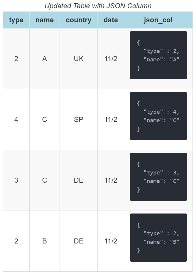
Our new field is called [json_col] and contains a simple JSON structure with the [type] and [name] for our data. In Snowflake, it is possible to directly query these entries:
SELECT
    json_col:type::number as type
  , json_col:name::string as name
FROM MY_TABLE
WHERE json_col:type::number = 2
;
In the exact same way, we can include these expressions in clustering keys:
ALTER TABLE MY_TABLE
CLUSTER BY (json_col:name::string as name, country, YEAR(date), MONTH(date), json_col:type::number as type)
;
This last example demonstrates how any of the following can be included in a clustering key:
- Base columns
- Expressions on base columns
- Expressions on paths in VARIANT columns
Keep in mind when defining clustering keys that it is certainly possible to go too heavy on the clustering. When too many elements are included in a clustering key, clustering the data can become too costly. Also, you may find the data is already clustered as well as it can be by the first field(s) in the clustering key. In this case, adding further fields to the clustering key will have no effect on query speeds but will still be costly to the system as it attempts to implement said further clustering.
A good principle to follow when choosing which fields should be included in a cluster key is to first consider which fields most commonly contribute to the filtering/WHERE clause in a given query. Secondly, you can consider which fields are used when joining to other tables.
Clustering Information
To assist with determining how well-clustered a table is, Snowflake has provided a system function called SYSTEM$CLUSTERING_INFORMATION. This function takes in a table name and a list of columns as inputs and outputs an overview of how well the table is clustered based on the list of columns. In effect, the list of columns is the clustering key for which the clustering information is being provided. You can thus use this function to determine how the data is clustered across several possible sets of columns, as well as potentially use this information to guide your final choice of clustering key for the table.
If no list of columns is provided, the function will instead return the clustering information for the table based on its current clustering key. If no current clustering key is defined on the table, the function will error. The function is executed using a SELECT statement, and it is important to note that both inputs are strings:
SELECT SYSTEM$CLUSTERING_INFORMATION('TABLE_NAME', '(COLUMN_1, COLUMN_2, ..., COLUMN_N)')
This function returns a single JSON object containing multiple fields that provide details on various aspects of the table’s clustering. Snowflake have described each of these in their own documentation. What I will do here is list Snowflake’s description (at time of writing) and provide further information:
cluster_by_keys
Snowflake’s description of this field:
Columns in table used to return clustering information; can be any columns in the table.
This is the list of columns that has been provided as an input to the function or the existing clustering key of the table if the input was left empty.
notes
Snowflake’s description of this field:
This column can contain suggestions to make clustering more efficient. For example, this field might contain a warning if the cardinality of the clustering column is extremely high. This column can be empty. For more information about how to cluster efficiently, see Strategies for Selecting Clustering Keys.
Snowflake have done well by including this field when it is relevant. When this field appears, it often provides guidance on whether or not clustering by the input clustering key is a good idea.
A standard and helpful message to see from these notes is that the cardinality of a particular field in the data is high and may result in expensive re-clustering. When seeing this message, it is recommended to consider alternative fields to use in the clustering key which may have a lower cardinality.
total_partition_count
Snowflake’s description of this field:
Total number of micro-partitions that comprise the table.
This field simply provides the total number of micro-partitions used to store the data for the table.
total_constant_partition_count
Snowflake’s description of this field:
Total number of micro-partitions for which the value of the specified columns have reached a constant state (i.e. the micro-partitions will not benefit significantly from re-clustering). The number of constant micro-partitions in a table has an impact on pruning for queries. The higher the number, the more micro-partitions can be pruned from queries executed on the table, which has a corresponding impact on performance.
This field is extremely useful when reviewing the clustering of a table. As this number increases, we can expect query pruning to improve and queries to execute more efficiently. Whilst not provided as a field by this function, I often find it useful to consider the total_constant_partition_count as a percentage of the total_partition_count. This provides a useful metric for what percentage of the data is clustered efficiently.
It is worth keeping in mind that this field should not be the only thing considered when reviewing clustering since it can lead to false positive scenarios. For example, our table could contain a boolean field which only ever has two values. We may find that the total_constant_partition_count is the full total_partition_count, which would suggest good clustering. However, any queries that filter on more than our single boolean field may not benefit from the clustering as much when pruning.
average_overlaps
Snowflake’s description of this field:
Average number of overlapping micro-partitions for each micro-partition in the table. A high number indicates the table is not well-clustered.
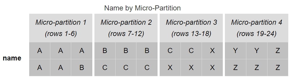
In this situation, an overlap is when the same value for a field appears in more than one micro-partition. Let’s return to our previous clustered example where we clustered based on the [name] field, specifically targeting this field:
After this clustering, we can see that each possible [name] value may still appear in multiple micro-partitions. Specifically, values B and C each appear in two micro-partitions:
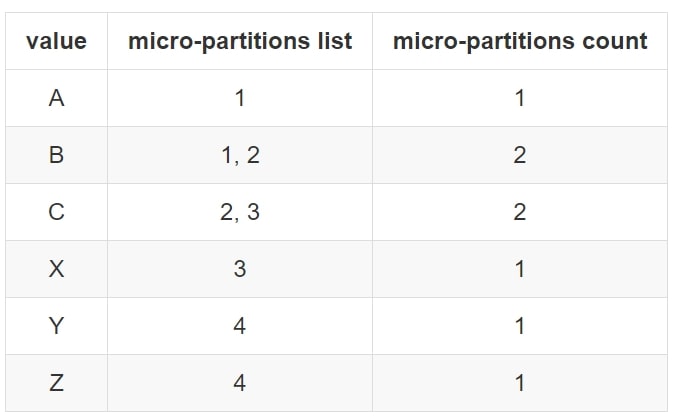
From a micro-partition perspective, we have four micro-partitions with the following overlaps:
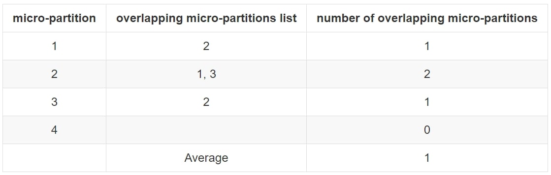
Here, we can see the average number of overlapping micro-partitions is 1 and thus the average_overlaps value from the SYSTEM$CLUSTERING_INFORMATION function will be 1.
average_depth
Snowflake’s description of this field:
Average overlap depth of each micro-partition in the table. A high number indicates the table is not well-clustered.
This value is also returned by SYSTEM$CLUSTERING_DEPTH.
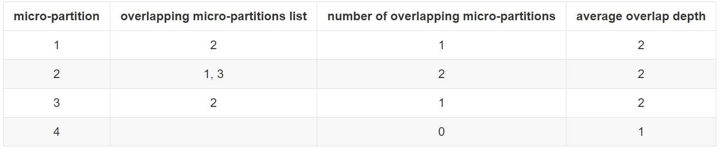
The overlap depth of a micro-partition is the average number of micro-partitions that an individual value may appear in when an overlap occurs. Let’s return to our previous example again where we have clustered by [name]:
The following table again demonstrates the overlapping micro-partitions, along with the minimum and maximum value in each partition. We can see that the values B and C both span multiple micro-partitions. We could represent this information differently:
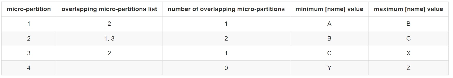

We can see from this diagram that we have three overlapping micro-partitions, but each value only overlaps with a single other micro-partition each time. Specifically, values B and C overlap. We could consider this in terms of values:
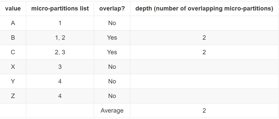
This tells us that whilst we have three overlapping micro-partitions (1, 2 and 3), the overlap depth is 2. Note here how values that did not overlap at all are not counted in the depth. The purpose of the depth is to understand more about overlapping data, and including non-overlapping values would skew this result.
The depth is still considered in terms of micro-partitions instead of values, so we aggregate this back to the micro-partition level:
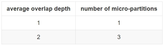
partition_depth_histogram
Snowflake’s description of this field:
A histogram depicting the distribution of overlap depth for each micro-partition in the table. The histogram contains buckets with widths of 0 to 16 with increments of 1. For buckets larger than 16, increments of twice the width of the previous bucket (e.g. 32, 64, 128, . . . )
This value takes the overlap depth for each micro-partition and plots it in a histogram. Let’s return to our previous example:
Here, our histogram is quite small, but it works for our simple demonstration purposes:
Example Output
Of course, real-world scenarios can be much more complicated than this. Snowflake provides its own example of a demonstration output of system$clustering_information that I have included below:
{
  "cluster_by_keys" : "(COL1, COL3)",
  "total_partition_count" : 1156,
  "total_constant_partition_count" : 0,
  "average_overlaps" : 117.5484,
  "average_depth" : 64.0701,
  "partition_depth_histogram" : {
     "00000" : 0,
     "00001" : 0,
     "00002" : 3,
     "00003" : 3,
     "00004" : 4,
     "00005" : 6,
     "00006" : 3,
     "00007" : 5,
     "00008" : 10,
     "00009" : 5,
     "00010" : 7,
     "00011" : 6,
     "00012" : 8,
     "00013" : 8,
     "00014" : 9,
     "00015" : 8,
     "00016" : 6,
     "00032" : 98,
     "00064" : 269,
     "00128" : 698
    }
}
Learning how to read and understand these diagrams takes time as there is a lot of information here. A question to ask yourself: Based on the information provided in the output above, do you think the table is well clustered? If so, why? If not, why not?
I won’t spoil the answer, but if you open this link to this example in Snowflake’s documentation, you can find the answer at the bottom.
The Cost of Re-clustering
In Snowflake, (re)clustering is performed in the services layer of the tool. This means that a virtual warehouse is not required, and Snowflake has its own way of keeping track of the credit cost. You can see this yourself in the Billing & Usage section of the Account area in your Snowflake environment, under the warehouse AUTOMATIC_CLUSTERING.
Automated Re-clustering Through Snowflake
This has been a pretty heavy-going post covering a lot of content, and we have covered WHY you may want to cluster a table and HOW Snowflake achieves this clustering. But we haven’t touched the best part yet–the part that separates Snowflake from other similar tools: Snowflake performs clustering automatically.
In most systems, processes must be put in place to re-cluster a table after data manipulation has occurred. Maybe one of the fields that contributes to the clustering key has had its valued changed, or maybe records have been added to or removed from the table. In most systems, somebody must either schedule clustering to occur (which may then run when not required) or manually apply re-clustering as and when it is deemed to be required.
Snowflake, on the other hand, uses an automated approach that is controlled by a single flag for each table. This flag is enabled or disabled using the following commands:
ALTER TABLE TABLE_NAME RESUME RECLUSTER;
ALTER TABLE TABLE_NAME SUSPEND RECLUSTER;
This is an extremely powerful tool as it takes the entire clustering process and removes all the irritating admin. The main thing to keep in mind though is that this can run away with you in terms of credit consumption if you are not paying attention to the number of objects. For example, if you create a clone of a table, that clone will default to have the same clustering information. Snowflake ensures clones disable automatic clustering by default, but it’s recommended to verify that the clone is clustering the way you want before enabling automated clustering again.
We can review the clustering for each table with either the SHOW TABLES command or through the tables view of the information schema. Specifically, the AUTO_CLUSTERING_ON field can tell you if clustering is enabled or disabled, and the CLUSTER_BY (SHOW TABLES) or CLUSTERING_KEY (information schema) field can be used to determine the current clustering key.
Summary
This post is an attempt to unlock some of the mystery behind clustering in Snowflake and explain some of the different ways this can be evaluated. There is a lot of content here, and I would recommend playing around with the functionality yourself to reinforce your understanding. Remember, you can make use of zero-copy cloning to give yourself a few test tables to play with and try out different clustering methods. As always, I’d love to hear your thoughts in the comments section down below. I hope you enjoy the rest of your day!