Machine learning is a vehicle through which we can maximize the value of data that already exists. Follow along as Elliott documents his first Udacity Nanodegree program and explores the possibilities machine learning provides.

When you ask someone a question, you likely have an idea of how the answer should be presented to you. For example, people will typically give you a specific time of day if you ask when they’re free for lunch. If you follow up by asking them if they’re a vegetarian, you’re probably expecting a yes or no answer.

Similarly, applying machine learning algorithms to real-world problems requires an understanding of how questions should be framed and the types of answers we expect to receive.

In previous posts, we explored regression and classification models: where regression is a good choice when seeking a numerical output and classification is a good choice when seeking a categorical or yes / no response. These approaches are great for predicting the value of a home (regression) or identifying fraudulent transactions (classification), but there are many real-world situations where neither approach is ideal.

Some Scenarios

Consider algorithms used for high-frequency trading on the stock market. This is a complex problem to solve, as the desired output from a model is more about finding the best course of action than it is predicting a numerical value or a binary outcome. Enter the reinforcement learning algorithm. This model can be used to assess the current state of the markets by being trained to take the optimal action given those market conditions. This approach provides additional value over a classification algorithm that is ignorant of the current state of the market (and therefore ill-equipped to identify the best course of action).

Alternatively, let’s consider a self-driving car as it approaches an intersection. How does reinforcement learning enable the car to select the optimal course of action to safely navigate the intersection and reach its destination?

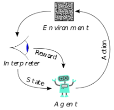
The short answer is that reinforcement learning relies on a list of predefined “states,” where each state has a series of actions that can be taken. You can think of a state as a series of attributes describing the environment, such as the color of a stoplight or the presence of oncoming traffic.

As the curators of the reinforcement learning algorithm, it is our job to define the state variables and the values contained within them. This is a delicate balancing act. Having too few state variables risks handicapping the algorithm by leaving it blind to important information about the environment. Inversely, having too many state variables risks making the algorithm difficult to train. This tradeoff reminds me of restaurant menus – having too few items on the menu limits the ability to deliver what customers want, but offering too many options is detrimental because it spreads the kitchen too thin.

Fig. 1: Illustration of reinforcement learning (image from Wikipedia).

Learning to Learn

The way the reinforcement learning agent learns is that it encounters a state, takes an action and then receives a positive or negative reward for that action. This process is repeated until (a) the learning agent has exhausted its training data, or (b) the learning agent completes an arbitrarily defined number of training trials. Ideally, once training is complete, the learning agent has a list of every possible state and a numerical reward associated with every possible action for each unique state. The decision process becomes a simple matter of selecting the action with the highest reward, given the current state.

There is a lot going on behind the scenes while the learning agent is trained. The reinforcement learning algorithm is controlled by various parameters, which alter how the “learning” is implemented. Keep in mind that “learning” in this context boils down to building a running tally of rewards for the actions available to any given state.

Q-Learning Explained

A common method for implementing this learning process is something called Q-learning. To keep this conversation from going off into the weeds, let’s focus only on the key components of Q-learning: learning rate, discount factor and exploration vs. exploitation.

The learning rate controls how quickly new information gained from the most recent training trials overwrites older information from previous training trials, while the discount factor controls whether the learning agent is trying to maximize short-term or long-term rewards. A learning agent with a relatively low discount factor will favor immediate rewards, and a learning agent with a relatively high discount factor will attempt to maximize long-term rewards.

Exploration and exploitation can be thought of as how adventurous the algorithm will be. We will loop back to this momentarily.

The Self-Driving Car Example

Let’s consider an example of reinforcement learning for a self-driving car in a simple environment where we only consider three things: the color of the street light, the direction of our destination and the presence of pedestrians in the walkway of the intersection. For simplicity, let’s assume our car is the only one in the intersection.

Our state variables would look something like the below table:

State Variable	Possible Values
Traffic Light	Green, Yellow, Red
Destination Direction	Forward, Right, Left, Backward
Pedestrians	Yes, No

 

The size of our state space is the number of unique situations which can exist, given every possible combination of our state variables. In this case, there are three street light colors, four possible destination directions and a binary value indicating if there are pedestrians in the intersection. The total number of states is therefore (3 * 4 * 2 = 24), meaning there are 24 states our model needs to consider. Four sample states are shown in the table below.

State	Traffic Light	Destination Direction	Pedestrians
1	Green	Backward	Yes
2	Green	Forward	No
3	Red	Right	No
4	Red	Left	Yes

 

Let’s say there are four possible actions our car can take: move forward, move right, move left and no movement. The actions and rewards associated with the first two states shown above could look like the table below.

State	Action	Reward
1	Forward	-1
1	Right	-1
1	Left	-1
1	Idle	0.2
2	Forward	0.2
2	Right	0.1
2	Left	0.1
2	Idle	-1

 

The training process may look something like this:

Trial	State Encountered	Action Taken	Reward Received
1	1	Right	-1
2	2	Left	0.1
3	1	Idle	0.2

 

Now let’s consider exploration vs exploitation. After these three trials, the learning agent has tried a few actions and has a few data points to help it make decisions when it encounters “State 1” or “State 2.” An algorithm that leans heavily towards exploration will tend to randomly select an action for any given state, whereas an algorithm that leans heavily towards exploitation will select the most rewarding action associated with any given state.

This raises the question: Why would we ever choose exploration overexploitation if exploitation chooses the most rewarding action? Let’s answer this question by taking a closer look the tables above.

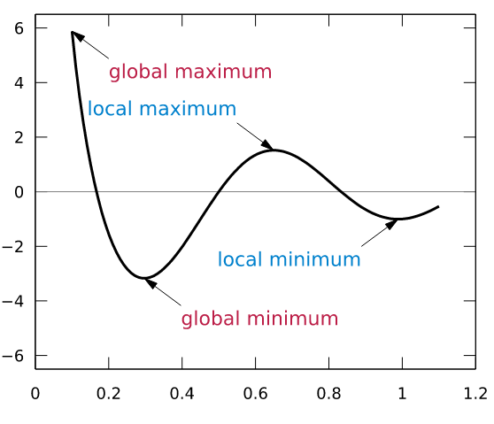
If the learning agent is running in exploitation mode, after three trials it will have learned that the best action to take for “State 1” is to remain idle and the best action to take for “State 2” is to make a left turn. However, we can see that the action that maximizes rewards for “State 2” is to move forward. This highlights why we want our learning agent to explore. If the learning agent leans too heavily on exploitation, then we risk getting stuck on a local maximum for our solution. In other words, if our learning agent spams the first positive reward, it encounters then we risk getting stuck in a sub-optimal solution that never branches out enough to discover even more rewarding actions.

Fig. 2: Exploration helps the reinforcement learning algorithm from getting stuck in a local maxima.

Ideally, the learning agent will try out all possible actions for each state throughout the training process. This is not possible if the learning agent gets tunnel vision on the first positive reward it finds.

Interested? Learn for Yourself.

Reinforcement learning is an excellent technique to employ when you have a firm understanding of the environment and situations you expect to encounter and you want automated decision making. If this post has piqued your interest in reinforcement learning, check out the Udacity Machine Learning Nanodegree smartcab project, where you can build your own reinforcement learning algorithm to train a (simplified) self-driving car.