In today’s data-driven landscape, artificial intelligence (AI) has permeated every corner of industry and technology. From personalized recommendations on streaming platforms to optimizing supply chains in manufacturing, AI algorithms are revolutionizing how we approach problems and extract insights from data. As organizations race to leverage this transformative power, platforms like Snowflake, known for their cloud data warehousing solutions, are at the forefront of integrating AI capabilities directly into their offerings.  

It is in this context that Snowflake Cortex emerges. Cortex provides capabilities that could be grouped into two main families: first, services that leverage large language models (LLM), and second, a fully managed machine learning model service that provides a wide range of ML-powered functions. In this article, we’ll explore the later and, specifically, one of its most popular ML-functions: forecasting.  

But fear not: the best part of Cortex is that all these goodies can be used with the simplicity that characterizes Snowflake and using a few simple SQL commands (or Python, in which case you can use Snowpark ML). Note that, at the time of writing this article, some of the functionalities of Cortex are still in private preview, so please consider this if you attempt to harness its capabilities in a production environment. 

Forecasting the Sales of Electrical Vehicles in Australia

For this article, I will be using a fictional dataset that represents sales of Electric Vehicles (EV) in Sydney. I have the number of units sold across several EV models for the last few years:

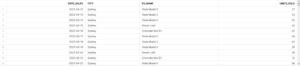
This is my “sydney_ev_daily_sales” table in Snowflake that includes sales for all vehicles. Let’s first see what sales look like for a single model:  

SELECT * FROM sydney_ev_daily_sales WHERE EV_NAME = 'Nissan Leaf';

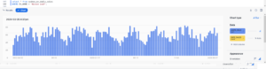
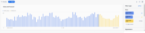
Using the awesome built-in visualisation feature of Snowsight, we can plot this data and observe the oscillatory pattern of our sales. Notice that the most recent record is for late March 2024.

Our objective: to forecast what the sales for Q2 2024 will be based on this data for one of the vehicles. Let’s get started! 

First, we want to slice our data to use a portion of it to train our forecasting model. So we’ll create a view with last year data for a specific model:

-- Create view containing the latest years worth of sales data for a given model:  

CREATE OR REPLACE VIEW last_year_nissan_sales_view AS ( 
    SELECT 
        TO_TIMESTAMP_NTZ(DATE_SALES) AS timestamp, 
        UNITS_SOLD 
    FROM 
        sydney_ev_daily_sales 
    WHERE 
        DATE_SALES > (SELECT MAX(DATE_SALES) - INTERVAL '1 year' FROM sydney_ev_daily_sales) 
        AND EV_NAME = 'Nissan Leaf' 
    GROUP BY all 
);

Important: You may have noticed that I casted my date field as a timestamp. That’s a requirement of the functions we’ll use later. Let’s now look at what do the sales for that given model look like: 

And here is when the magic begins. Our goal is to estimate the sales for this vehicle. To do so, we’ll simply use the keyword FORECAST, a built-in function capable of running time series predictions. The syntax is pretty simple, but, in essence, it takes in three parameters: a) what data are we using to train the model (it can be a view or a table), b) what is the timestamp column and c) what column are we trying to predict the value of.  You can see below how I populated it:  

-- Build Forecasting model; this could take a few seconds 

CREATE OR REPLACE SNOWFLAKE.ML.FORECAST nissan_sales_forecast ( 
    INPUT_DATA => SYSTEM$REFERENCE('VIEW', 'last_year_nissan_sales_view'), 
    TIMESTAMP_COLNAME => 'TIMESTAMP', 
    TARGET_COLNAME => 'UNITS_SOLD' 
);

While the syntax is simple under the hood, this is a computationally expensive query: using a standard warehouse, you may need to wait several seconds for this to command to execute. For such scenarios, we could well consider using a Snowpark-optimized warehouse, but the standard warehouse will do for the purposes of this article. Also, before using this technology, please bear in mind some of the considerations outlined by Snowflake, including its metadata usage policy. 

Once this command is executed, our model has been trained and is ready to be used. Let’s first test the waters: using the CALL command, I will pass 10 as the number of periods I want the model to forecast (that is, number of timestamps). This, in turn, will expose some additional bits of the model: its lower and upper bounds. In other words, the range of values that your model is predicting your sales to fall within:

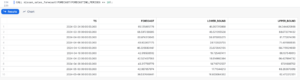
Let’s run it again to run a prediction for a longer period. This time, however, we will invoke the model but also scan the last query so we can store the results in a new table that will contain our predictions for our EV. Make sure you run these two commands together:

-- Create predictions, and save results to a table. Run these two commands together to store results 

CALL nissan_sales_forecast!FORECAST(FORECASTING_PERIODS => 30); 

CREATE OR REPLACE TABLE nissan_predictions AS ( 
    SELECT 
        * 
    FROM 
        TABLE(RESULT_SCAN(-1)) 
);

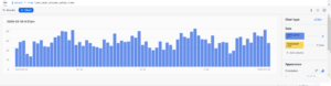
And that’s pretty much it. We can now visualize our actual and forecasted sales by running a simple UNION ALL and, again, using the awesome built-in features from Snowflake: 

-- Visualize the results, overlaid on top of one another 

SELECT 
    timestamp, 
    UNITS_SOLD, 
    NULL AS forecast 
FROM 
    last_year_nissan_sales_view 
UNION ALL 

SELECT 
    TS AS timestamp, 
    NULL AS UNITS_SOLD, 
    forecast 
FROM 
    nissan_predictions 
ORDER BY 
    timestamp asc;

And sure enough: we see that our models have projected sales for Q2 2024. Note: you can adjust the visualization on the right-hand side to add the FORECAST column if it’s not plotted by default: 

Here, we have only scratched the surface, but as you can see, with a few basic commands you can train, deploy and evaluate ML models for time-series forecasting tasks. Whether predicting sales trends, anticipating demand fluctuations or optimizing resource allocation, Cortex can equip your team with the tools that you need to extract valuable insights from time-series data.