
Machine learning is a vehicle through which we can maximize the value of data that already exists. Follow along as Elliott documents his first Udacity Nanodegree program and explores the possibilities machine learning provides.
Welcome back! Today we’re going to trace my steps through the first few weeks of the Machine Learning Nanodegree program. If you missed the first post, check it out! So far, I’m feeling good about my experience and I’m excited to share what I’ve learned so far. This will likely end up being the longest post in the entire series, since this Nanodegree program wastes no time in dropping knowledge on you from the start.
Here is the agenda for this week’s post:
- Give you an idea of what the Nanodegree program is like.
- Introduce several crucial concepts that will lay a foundation of the ins and outs of machine learning.
- Describe my experience with the first project.
But before we do all of that, I want to take a moment to share my thoughts on machine learning in general.
What Is Machine Learning?
One of the many aspects of machine learning that intrigues me is that there is no one-size-fits-all solution. Instead, we are provided a great number of tools, each equipped with a unique array of strengths and weaknesses. The quality of the models we build is equally dependent upon our mastery of these tools and our knowledge of the underlying problem needing to be solved.
Machine learning is not necessarily about putting a computer in charge of making decisions for us. I’d argue it’s about processing information in a way that leads us to the best possible decision. An important choice you’re faced with each time you solve a problem with machine learning is which algorithm to use:

Each algorithm’s performance will vary greatly depending on the nature of the problem. This makes perfect sense if you consider other situations where you would choose one option over another. For example, today I drove a car to work, yesterday my feet carried me to a nearby restaurant and next month a plane is flying me to another part of the country to visit my family.
We use these different modes of transportation interchangeably because each one takes us from where we are to where we want to be. Typically, the vehicle we choose to take is the one that’s most efficient given the circumstances.
Driving to work is the right call for me, because it gets me there faster than walking and it’s more efficient than flying four tiny miles. Not to mention, financing a private jet would vaporize my bank account. But even though driving is a great way to get to work, it’s complete overkill for me to drive to a nearby restaurant that doesn’t have a parking space for my car. So, for that situation, it’s best that I walk.
To summarize, we’re all well versed in solving everyday challenges. My goal is to plant the idea that on some level, this is not so different from how we approach machine learning. We see a problem, we consider the toolbox available to us and we select the most appropriate tool for the job. The biggest hurdle for us as we explore machine learning will be getting comfortable with a new set of tools.
Nanodegree First Impressions
Within minutes of beginning the program, I was introduced to my mentor. Each student has one and, for a short duration of the program, they are available to help you set achievable goals or just be helpful in general. I didn’t speak with my mentor all that much, but I’m not really a social butterfly when I’m knee deep in course content.
Having said that, I’m a huge fan of the program’s Slack workspace. Through Slack, students are provided numerous invaluable resources that are organized and easily accessible. I immediately felt like I was part of a larger community. It’s important to have an outlet for asking questions, however trivial or complex they may be. This open transfer of knowledge adds a ton of value and I’ve been cherry-picking information from various Slack channels that I might never have found or sought out on my own.

The structure of the program is straightforward enough. Each lesson is delivered to you through a series of videos, many of which have quizzes that go along with the content. These prepare you for projects that will test your understanding of the theory.
I was pleasantly surprised by the detail and effort that was put into providing feedback on my project submissions. I’ll discuss this in more detail later on. One project I’m particularly interested in is the capstone project. It’s an open ended task where you must identify and solve a problem of your own choosing. Decisions, decisions.

Key Takeaways & Concepts
There are so many things we could cover here that I believe it’s important to focus on the most crucial items rather than spend an eternity summarizing every concept relevant to machine learning. For example, I don’t think it would be very productive for me to explain the difference between supervised and unsupervised learning or discuss the different methods of measuring residual error. Instead, I’ll dive into the important topics surrounding machine learning.
A Simple Kind of Model
In the context of this discussion, you can use the image below to visually compare an example of a complex model to a simple model. In the image below, let’s assume the blue line represents a complex model, while the green line represents a simple model:
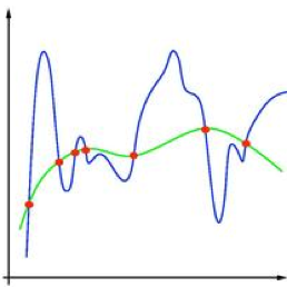
Models don’t have to be incredibly complex to be effective. In fact, an over-complicated model will often be outperformed by a simpler model. Our goal with machine learning is to generalize the functions that govern the true relationships between our inputs and outputs. We will never have a perfect model, but that doesn’t mean we can’t make good predictions. Complexity is not inherently bad, but it is important to remember increased complexity is not a golden ticket to building a better model.
Overfitting and Underfitting
The image below is a good visual interpretation of how underfitting and overfitting can look:
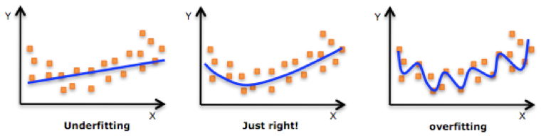
To explain overfitting and underfitting, let’s consider a situation where I’m predicting how the plot of a cheesy, sci-fi flick will unfold (this is not a rare thing to witness, by the way). Within five minutes of the movie starting, I might casually announce that a character’s military fatigues are a sure sign that a top-secret experiment will go awry.
Horrific creatures will then escape and a dislikeable character will quickly be annihilated by the rogue science experiment. But then, a handsome hero will team up with a strong independent heroine to narrowly escape death and win the day. Extra points if there’s a nerdy scientist for comedic relief. For argument’s sake, let’s assume this is a decent generalization of a sci-fi movie plot.

Above: Image of said cheesy, sci fi movie.
Now, suppose I add complexity to this model by declaring that the hero’s name is John and the heroine’s name is Jane, because another movie used those names. This model would be in danger of being overfit. While these names could be accurate for one film, it’s unlikely that every sci-fi movie will recycle those names. This model is overfit because it is too married to the data it was trained on and will not generalize well when applied to other films.
On the other hand, if the model is oversimplified to only predict that the movie will feature a breathable atmosphere and green socks, then this model is in danger of being underfit. This underfit model also does a poor job of generalizing the overall trend of cheesy, sci-fi movie plots. You could argue that underfit models aren’t specific enough since they don’t perform well on training data.
Training, Validating and Testing
Fortunately, we have a good way to avoid overfitting or underfitting our models. By separating the data into training and testing sets like in the image below, we allow models to learn underlying patterns about training data before evaluating how well the predictions perform on testing data:
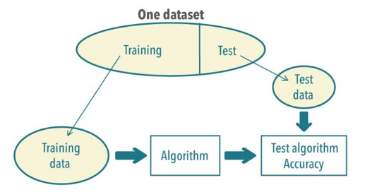
However, having only one shot at training and testing your model doesn’t provide a lot of wiggle room to find the best solution. That’s why we also have tools available to split our training data into smaller portions of training and validation sets. Validating our model is a great way to evaluate model performance without laying a finger on the test data.
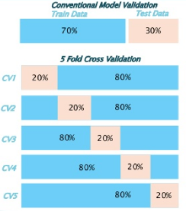
After this stage, you should have a fine-tuned model that can be evaluated against your pristine, untouched testing data. The figure below provides a glimpse into the K-Folds cross-validation technique, a popular approach when building robust models:
It’s important that you do not test your model on the same data it was trained on, because this is a recipe for overfitting. You don’t want your model to be so fixated on the training data that it overlooks the true relationship between inputs and outputs. We want our models to learn from the training data so that they will become good at generalizing. This allows them to make useful predictions about future data that the models have not yet seen.
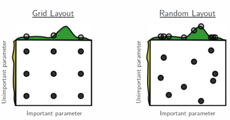
Another important point to keep in mind when cross-validating a model is parameter tuning. Depending on the algorithm you’re using, there are essentially different knobs you can twist and turn to change the way the algorithm behaves. You could tune your model by tediously altering these parameters manually, but there’s no need for that. Just as we have tools for splitting our data into training and testing sets, we also have techniques such as grid search and randomized search that help us find the sweet spot for our model parameters.
The figure below shows how various combinations of parameter values can be tuned to build an optimized model. Take this image with a grain of salt, since it is borrowed from a visual demonstration of how a random search process can sometimes have benefits over a grid search process:
Accuracy Isn’t Everything
When judging the performance of your model, there’s a lot more to consider than its accuracy. To be clear, accuracy tells you what percentage of your predictions are correct. To understand why this doesn’t tell the whole story, we need to introduce another tool called the confusion matrix. A confusion matrix looks at your model’s predictions and stacks them up against the true labels in the testing set. For example, look at the figure below:
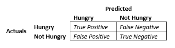
Depending on the problem you’re solving, your model’s accuracy may not be as meaningful as its ability to minimize false positives or false negatives. For example, if you have a model that predicts whether customers will respond to a direct mail promotion, then you probably only want to send promotions to customers who are likely to respond. This means the model should minimize false positives. If you’re predicting engine failure on an aircraft, then you probably don’t want to let engine failures slip by undetected. In that case, the model should minimize false negatives.
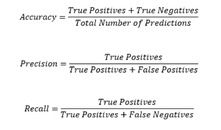
The metrics we use to describe our model’s ability to minimize false positives or false negatives are precision and recall. Having high precision means your model is rarely going to predict something is true if it’s not. Having high recall means your model will rarely predict something is false when it’s true. The figure below shows how accuracy, precision and recall work:
I like to think of this in terms of playing poker. If your model has high precision and low recall, then it plays a tight and conservative game, only making bets when it has a very good hand. This model doesn’t mind folding a decent hand every now and then, because it only goes all in when there’s a high probability of winning. If your model has high recall and low precision, then it plays fast and loose, and would rather chase a straight or a flush than fold on an opportunity to win the pot.
In the real world, this poker analogy breaks down a bit under scrutiny, because we have neglected to mention that precision and recall never exist independently of one another. Our model could have low precision and low recall, high precision and high recall, or anything in between. This brings up an important question: How can we assess the quality of our models in terms of both precision and recall simultaneously?
We could simply average precision and recall, but that’s not a good idea. Imagine a model that has zero precision (everything we predict as true is false), but perfect recall (never predicts something to be false when it is in fact true). This is a terrible model, but the average of its precision and recall score would be 50%. Based on how useless such a model would be, we don’t want to be charitable and give the model such a high score when it should be rated closer to 0%. So, what can we do?
This is where the F1 score comes in. The F1 score gives us the harmonic mean of precision and recall. If one of the two metrics is very low, then the overall score will be low. In the example above, the F1 score would be 0%, which helps us learn that the model is garbage. The actual formula looks like this:
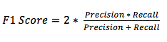
Both precision and recall must be high for the F1 score to be high. If either metric is low, then it will drag down the entire score more dramatically than a standard average would.
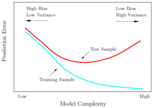
Bias and Variance
One last topic that we absolutely can’t leave out is the bias-variance tradeoff. If I’ve learned anything during the first week of this program, it’s that building a good machine learning model is one big balancing act. I imagine it’s like coaching a soccer team: If you put extra players on offense, then your defensive position is weaker. If you pull players back into defensive positions, then you’re not going to have as many opportunities to push the offensive counterattack.
A similar game of tug of war exists with bias and variance. To loosely define the two terms, bias measures how badly your model misses the relationship between inputs and outputs. Variance measures how sensitive the model is to the training data. In other words, a model with high bias is inflexible and is likely underfit, while a model with high variance is so flexible that it bends over backwards to fit the training data and is probably overfit, like in the image below:
To build a robust model that does a good job generalizing the underlying trends in our data, we must strive to find the sweet spot in the bias-variance tradeoff. We don’t want the model to be so stubborn that it can’t bend a little to fit the training data. We also don’t want the model to be so eager to please that it moves heaven and earth to fit itself to every single value in the training set. We want something in between those two extremes and that’s why we play the balancing act.
Putting Theory to Practice
So far in the program, I’ve completed one official project as well as two smaller projects. The two smaller projects were so heavily guided that I won’t discuss them beyond mentioning that they showcased the usefulness of decision trees and the Naive Bayes classifier. With that out of the way, let’s take a closer look at the program’s first project: predicting Boston housing prices.

Without unloading all the details, this project involves building a model that allows us to accept certain features of a home as input and provide an estimated value of the home as output. To build the model, we need to use the new tools that we discussed earlier and select an algorithm suitable to this type of problem. We also need to split the data into training and testing sets, fit the model to the training data, cross-validate the model, and then finally make our predictions and evaluate the results.
Because this project is the first in the program, the technical pieces are spoon-fed to you, but having a functional model doesn’t mean that you understand what makes the model tick. This became very clear to me when I received feedback on my first project submission. The person who reviewed my submission was extremely knowledgeable. They told me I needed to rethink some of my answers to the questions throughout the project, since the topics covered are crucial building blocks required to master the overall material.
This was a pleasant surprise for me. The feedback came with suggested resources to help fill in the gaps of my theoretical knowledge and it also highlighted areas where I had done well. I was not expecting this level of attention and detail in an introductory project submission. Hats off to the Udacity reviewers for setting the bar high!
My second attempt improved upon the first and passed with flying colors, but my reviewer still provided valuable insights and suggestions. I’m looking forward to going through this process again for the next project, which I’m sure will be more challenging. I think this hands-on intersection of theoretical knowledge and practical implementation is critical to the learning process. This is the difference between half-baked, self-taught resources and a quality program that doesn’t take shortcuts to provide an educational service.
Let’s Recap!
In the first week of the program, I’ve learned a lot and I’m excited for what’s next. I’m getting more and more comfortable with the tools that do most of the heavy lifting in machine learning. Plus, I’m working on supplementing my knowledge by accompanying the applied exercises with outside reading material. Let’s recap some of the key takeaways I’ve absorbed from these first weeks:
- There is no silver bullet when it comes to choosing a machine learning algorithm, so choose wisely.
- Keep things simple when possible and weigh the benefits of complexity with the costs of overfitting.
- Cross-validation is a great way to efficiently take steps towards the best possible model.
- Accuracy does not exist in a vacuum. You must also consider precision and recall.
- Strive to minimize bias and variance simultaneously.
That’s it for now! I’ll be back again in a week or two with another update.