When dealing with large data sets speed can be crucial. Fortunately, Alteryx Predictive Tools utilizes R to provide a seamless framework to extend the toolset that comes with Alteryx Designer. This means that Alteryx users benefit from all of the powerful packages developed by the R community to add functionality and increase the speed of their modules.
If you have Alteryx Predictive Tools installed, you can use the R Tool to execute R code in your Alteryx module. While it is by far the simplest way to use R with Alteryx, it may not always be the quickest way to analyze your data when dealing with larger data sets.
For Alteryx and R to be used in tandem, there must be data passed between the Alteryx Engine and R. This data handoff can be complicated, so Alteryx has developed a custom package called AlteryxRDataX containing functions that take care of this transfer for you. Many of these functions can be auto-populated from a drop-down menu in the R Tool configuration:
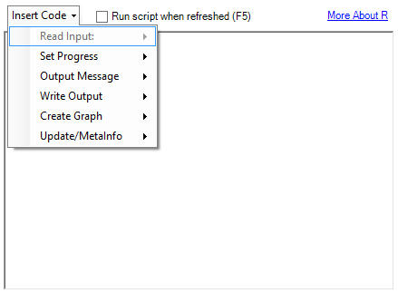
These functions work reliably and are easy to understand. Unfortunately, I have seen some performance issues with larger data sets. Let’s explore the benefits substituting the Run Command Tool for the R Tool to take advantage of some speedy functions in a couple of popular R packages.
In order to follow along, you will need to have Alteryx Predictive Tools. Visit the Alteryx Download page to get Predictive Tools and see the list of R packages that come standard with it.
Installing the Necessary Packages
To get started, there are three R packages we need: dplyr, data.table and RSQLite. Because CRAN only keeps source versions of older packages and not binaries, I would recommend using the mirror at Revolution Analytics to download the packages.
The primer on how to install new packages into your Alteryx R library can be found here.
However, since we are using a different R repository and installing multiple packages, I have provided the modified code below. Open Alteryx, drag an R Tool into the canvas and paste the code block below into the tool configuration. Running the module should install the packages, but be aware: The directory of your R library may be different than mine. It will be located wherever you have Alteryx installed inside the directory R-
pkgs <- c('dplyr', 'data.table', 'RSQLite')
# your library path may be different
alteryx.lib <- 'C:/Program Files/Alteryx/R-3.1.3/library'
revo.cran <- 'http://cran.revolutionanalytics.com'
for (i in 1:length(pkgs)) {
  if (pkgs[i] %in% rownames(installed.packages(lib.loc = alteryx.lib)) == FALSE) {
    install.packages(pkgs[i], lib = alteryx.lib, repos = revo.cran)
  }
}
If you receive a message that the directory is not writeable, then you probably have the administrator-required version of Alteryx installed. Running Alteryx as an admin will solve this issue.
Testing the Alternatives
I have provided three sample modules so that you can follow along with the testing. Download those and other relevant files here. The first module (r-tool) is simply an Input Tool, an R Tool and a Browse. The code run by the R tool is two simple lines:
df <- read.Alteryx("#1", mode="data.frame")
write.Alteryx(df, 1)
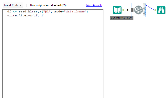
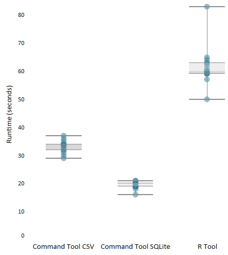
This module is the absolute minimum required to use the R Tool. Pass data from Alteryx to R for processing and then back to Alteryx. Run it and you will see that it takes a considerable amount of time simply to pass data from Alteryx to R and back again. That is without any other calculations performed inside of R. Repeated testing gave me an average run time for this model of about 62 seconds.
Let’s look at a couple of ways to speed this process up using the Run Command Tool to run a .R file with Rscript.exe.
The second module (command-tool-csv) is an Input Tool, a Run Command Tool and a Browse. To run this module successfully, you may need to change Command from C:Program FilesAlteryxR-3.1.3binx64Rscript.exe to the location of Rscript.exe in your Alteryx installation just as we did above with the R library.
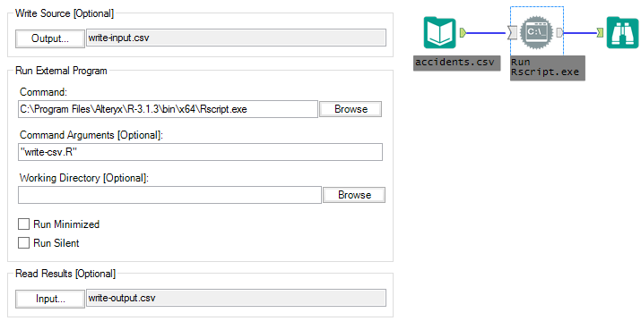
With this module, instead of passing data from Alteryx to R using the commands provided by Alteryx in the R Tool, we are writing the data stream to a CSV (Write Source in the Run Command configuration is write-input.csv) and then reading that CSV inside of the write-csv.R file run using RScript.exe. The write-csv.R file is simply a text file with the following R code:
library(methods)

#read data from Write Source in Alteryx into R
t <- data.table::fread('./write-input.csv', sep = '|')

#write csv to be read in Alteryx by Read Results
write.table(t, './write-output.csv', quote = FALSE, sep = '|', row.names = FALSE)
Again, this is the absolute minimum required to run R in tandem with Alteryx. Pass data from Alteryx into R for processing and back again. Except this time, instead of using the functions provided by Alteryx, we are writing a CSV of the Alteryx data stream and then reading it into R with the speed of fread() – a data.table function. Once the data is inside of R, we write it back to a CSV that will be ingested by Alteryx (Read Results in the Run Command configuration is write-output.csv). Unfortunately, there isn’t currently an fwrite() function, so we will use the R standard write.table(). Testing on this module shows an average of 33 seconds which is a considerable performance increase.
The third module is able to shave another 14 seconds off of the average run-time by utilizing Alteryx’s ability to read from SQLite. This module looks similar to the second, but it has two key differences:
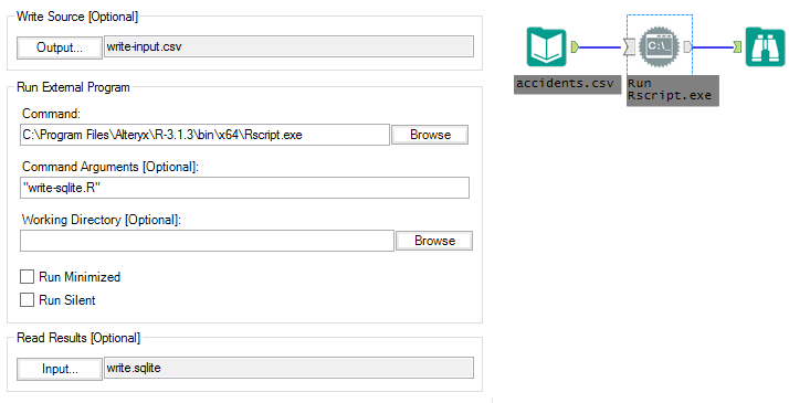
Instead of reading write-output.csv into the Alteryx data stream from R, ‘Read Results’ in the Run Command configuration now points to a table called “output” in a SQLite database, write.sqlite. Inside of the Rscript, instead of using write.table() to create write-output.csv, we use copy_to() from the dplyr package to write the output to SQLite:
library(methods)

#read data from Write Source in Alteryx into R
t <- data.table::fread('./write-input.csv', sep = '|')

#establish connection to sqlite database
sl <- dplyr::src_sqlite(path = './write.sqlite')

#drop existing output table and recreate with the new data to be read by Alteryx
if(dplyr::db_has_table(sl$con, 'output')) {DBI::dbGetQuery(sl$con, 'DROP TABLE "output"')}
invisible(dplyr::copy_to(sl, t, 'output', temporary = FALSE))
Testing on this module shows an average of 19 seconds runtime. Below you can see the distribution of the runtime for all three modules:
Moving Data Takes Time
In a real-world scenario, we would be doing more than passing data back and forth between Alteryx and R. Between the read and write steps there would be several lines of data manipulation logic. The examples here are a base-case experiment for speeding up data transfer between Alteryx and R. I’ve seen this implementation save hours on processes for clients.
Aside from a few tricks you’ve picked up along the way, the major takeaway is, in any use case, always understand where data lives, which applications are moving data around and keep your calculations as close to the data as possible.
