
This blog post is Human-Centered Content: Written by humans for humans.
I recently kicked off a blog series for people (like me) coming to Sigma from a Power BI background. If you haven’t had a chance to read the first blog in this series, that’s a good place to start. To keep building on that thread, this blog is going to cover one of my favorite topics: Data modeling.
One of the many reasons I’m grateful for my Power BI background is the early introduction the platform provided to star schema modeling. My early days fumbling around, trying to replicate Excel’s lookup patterns and navigate many to many relationships forced me to engage with modeling challenges and learn (often the hard way) what best-practices look like.
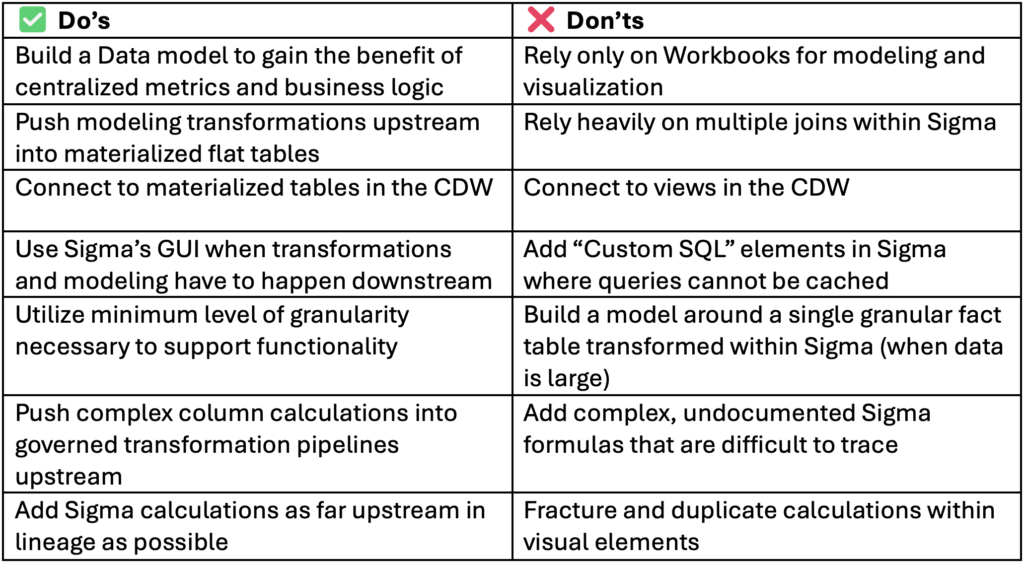
Over time I grew familiar with a running list of Power BI do’s and don’ts, to name a few:
Power BI Do’s and Don’ts
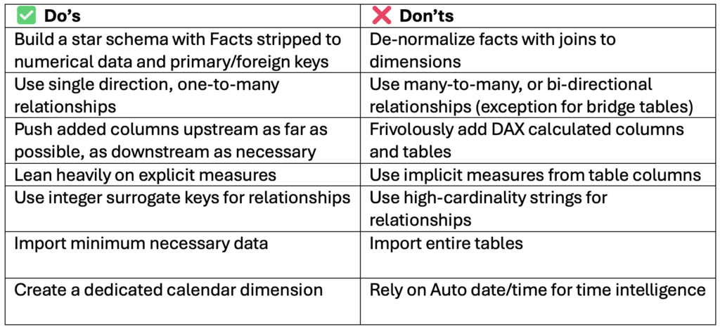
Ask a seasoned Power BI developer for a new model column, and they will ask you how it can be a measure.
As I began learning Sigma, I found that the rules of the game are different. The list of best practices isn’t the same. Much of the functionality appears similar at first glance, but when fully unpacked contains some meaningful differences worth noting.
For instance, adding tables and columns is not the same as Power BI where these additions get loaded into memory and increase the RAM used to store the semantic model. Instead, Sigma’s added tables, columns and metrics are more like Power BI’s measures, adding compute at query time.
There are similarities overall, but fundamentally Sigma is a different modeling paradigm. Ultimately Sigma operates best on pre-joined, flat tables instead of Power BI’s beloved star schemas. That’s the topic for today — let’s dive in.
How Sigma Modeling Looks Pretty Similar
Sigma’s platform offers functionality that parallels much of what semantic model development looks like in Power BI:
- Create a Data Model (separate artifact than a Workbook)
- Connect to tables
- Build relationships
- Add metrics
- Connect multiple downstream Workbooks to one Data Model
If you stopped there, you might get the impression that these are two similar BI tools that offer a comparable modeling experience. From a high-enough level, that’s an accurate take.
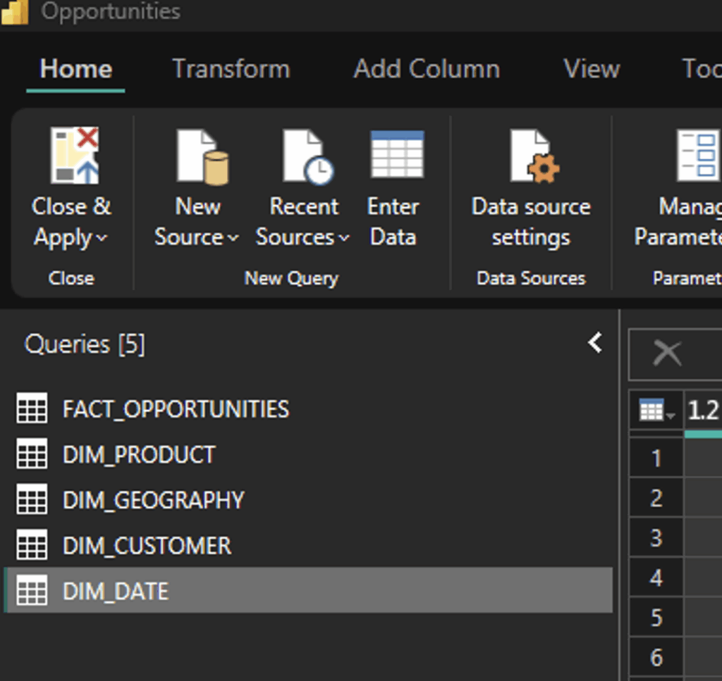
To further explore how these two tools align, I’ll be using a synthetic data set with Salesforce opportunities, and a set of related dimension tables to do some modeling. The goal for this simple analysis will be to create a SUM calculation for the Software Amount in our opportunity data.
The primary fact table, FACT_OPPORTUNITIES contains a PRODUCT_SKU that is a foreign key to the DIM_PRODUCT table, where a PRODUCT_FAMILY category lives to categorize Software.
Power BI Modeling
In Power BI, we take the following steps:
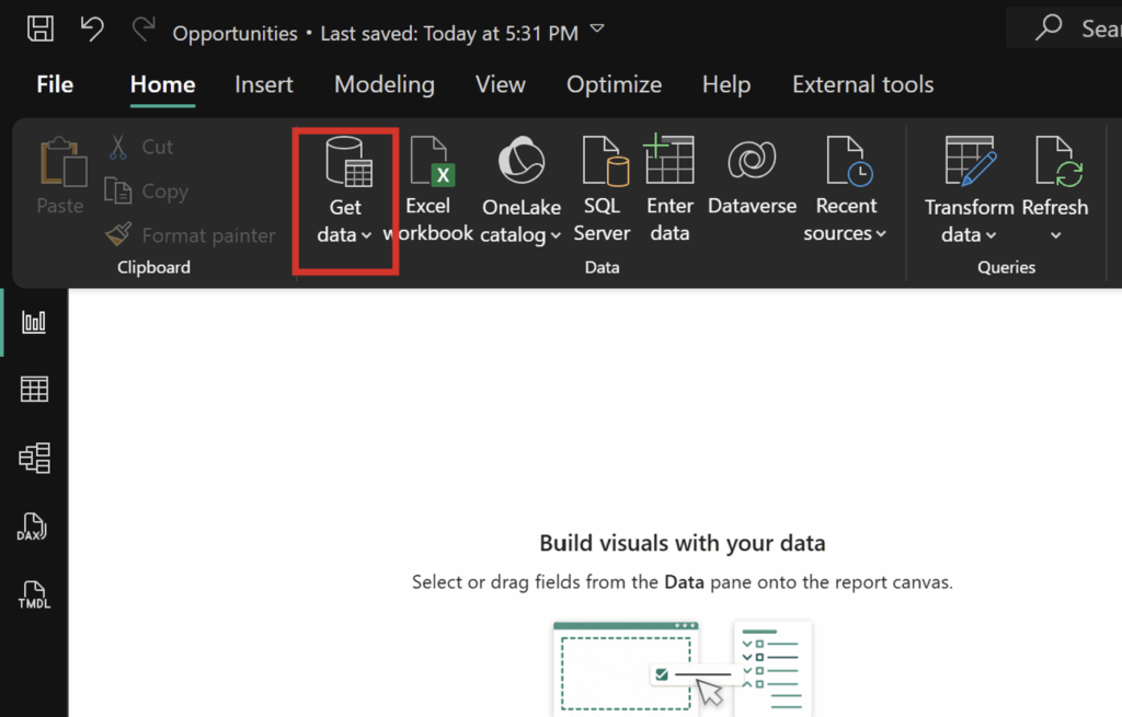
- Open up Power BI Desktop and navigate to the “Get data” dropdown:
- Connect to tables in Power Query and import into my semantic model:
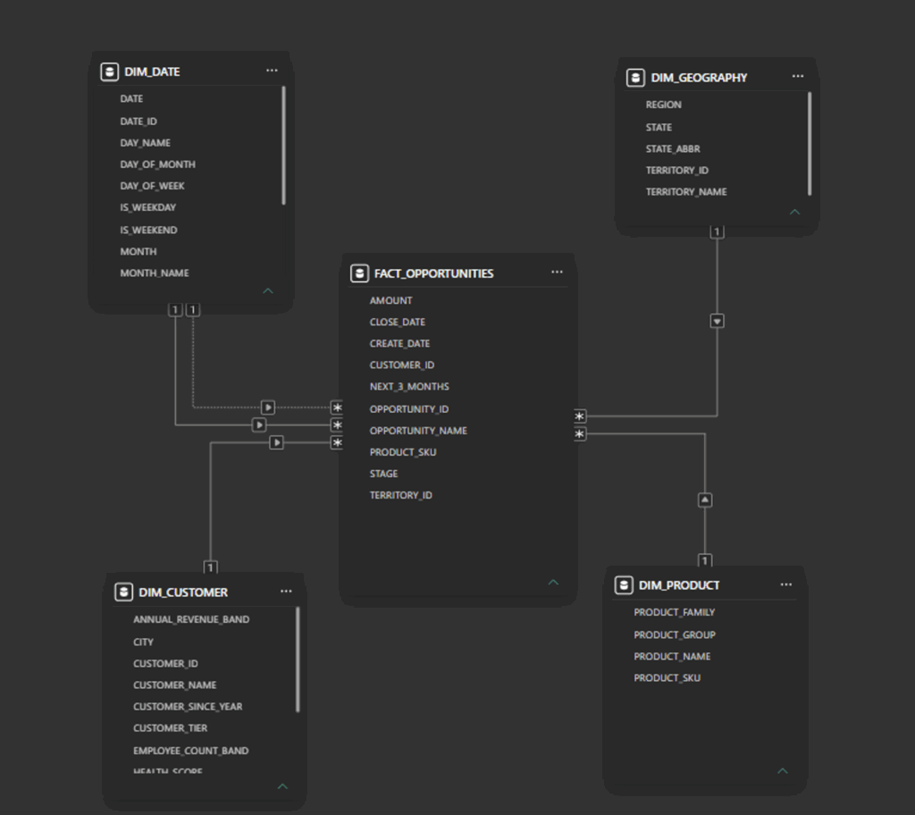
- Add single-direction, one to many relationships from the dimension tables to the opportunity table:
- Add a DAX Measure with the Software calculation (not a column – no weight added to the model):
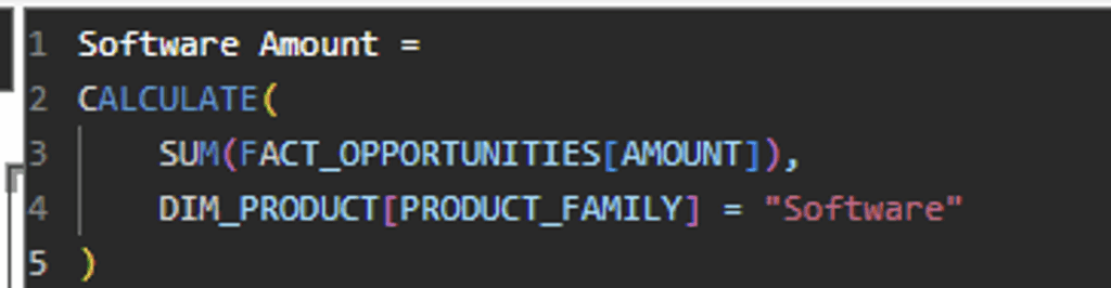
Note that the DAX measure allows references to multiple tables in this calculation (which behind the scenes is running a join).
Sigma Modeling
The process in Sigma looks pretty similar, until the last step:
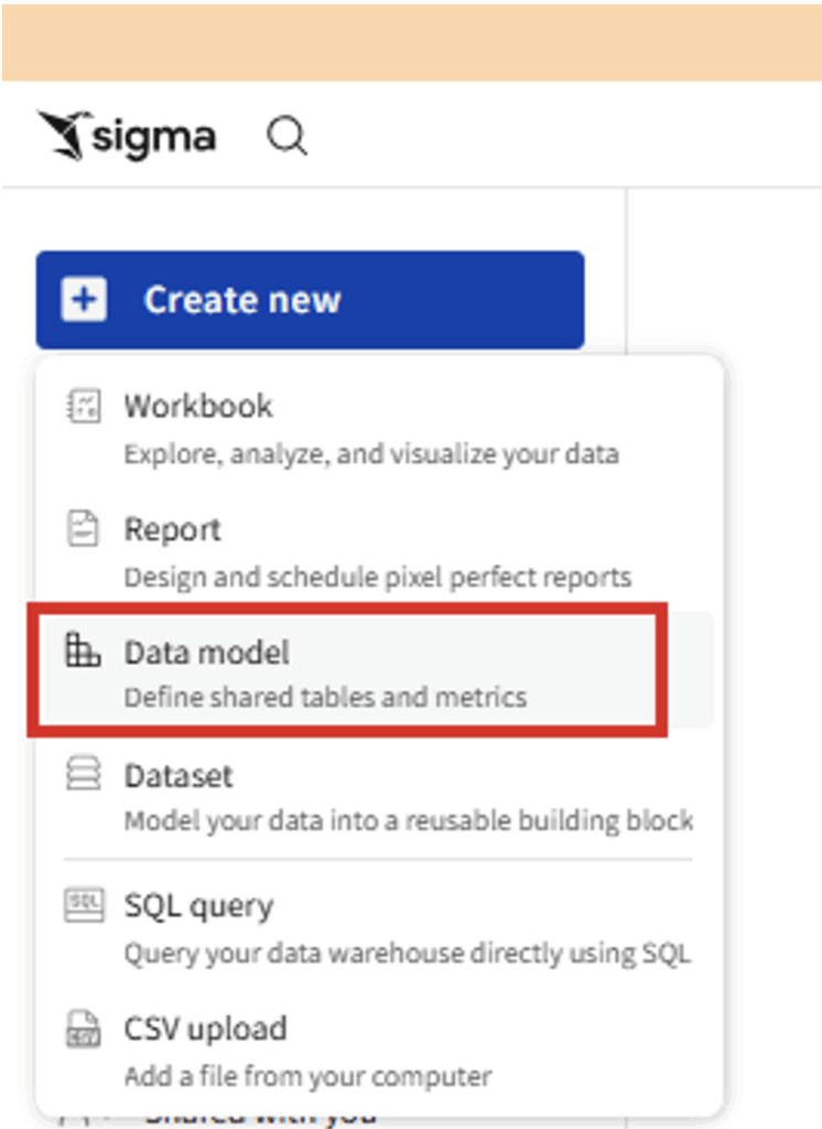
- Create a new Data model:
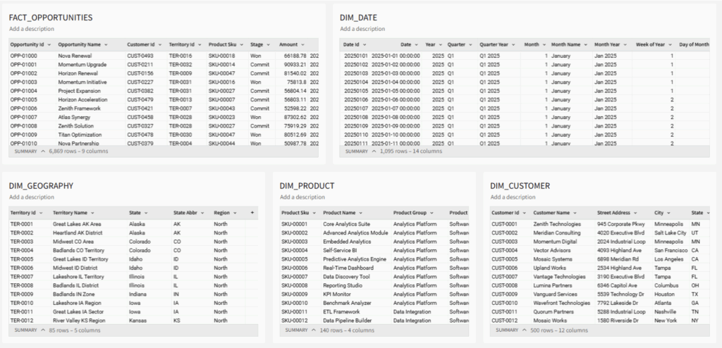
- Create Table elements connected to our source tables:
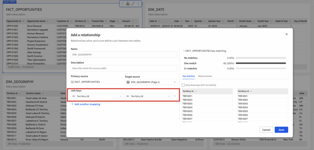
- Add relationships from the FACT_OPPORTUNITIES out to each dimension table:
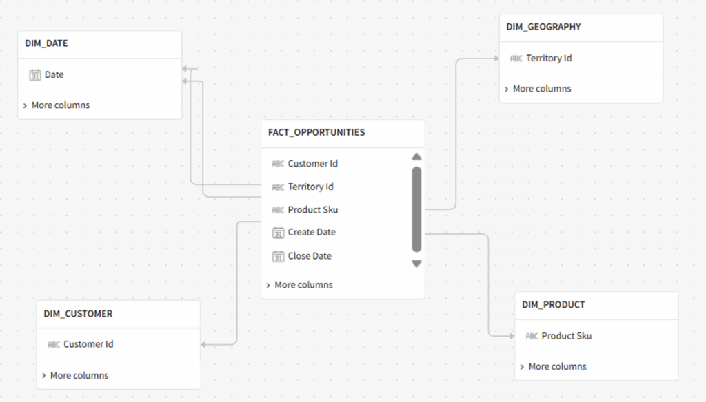
Add Metrics, which must be added within a single table in Sigma. Since we need to do a SUM, I will need to use the FACT_OPPORTUNITIES table containing the Amount field:
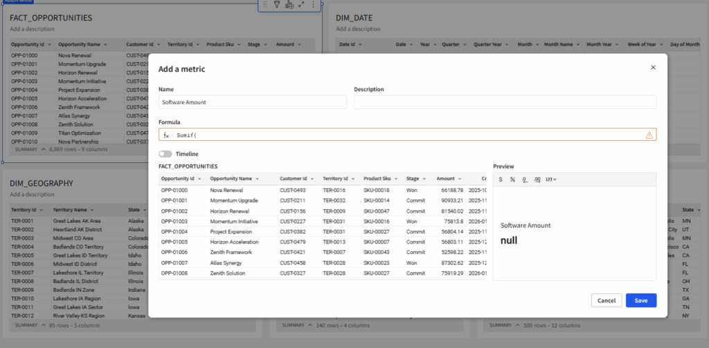
⚠️ This is where things start to get different. In the “Add a metric” GUI, I get a reference for my available columns beneath the formula bar. I can see the “Product SKU,” but not the “Product Family” I need to support this calculation. Relationships function quite differently in Sigma compared to Power BI — they are actually potential joins waiting to be activated.
This may seem like a small detail, but to a developer entrenched in Power BI modeling coming into Sigma, this cascades into an entirely different modeling paradigm.
How Sigma Modeling is Actually Pretty Different
In order to utilize this join, I first need to create a child table from FACT_OPPORTUNITIES, navigate to this child table’s Properties, and look in “Available columns:”
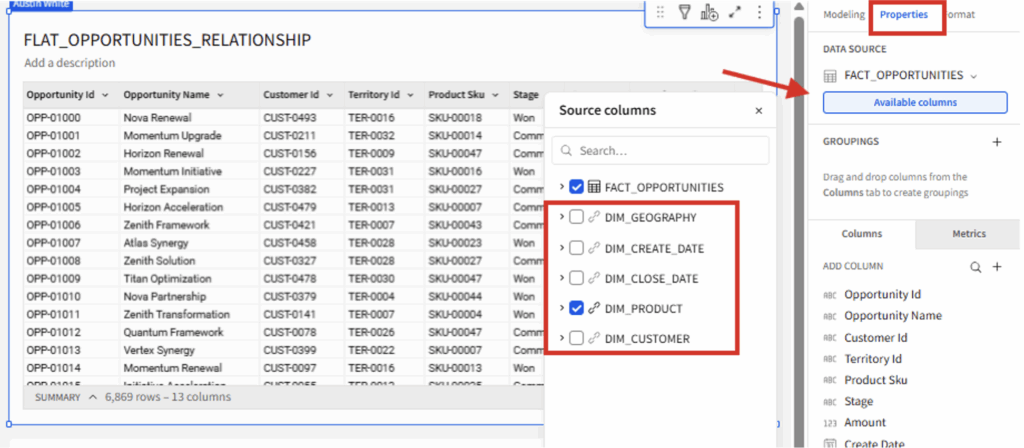
All of the tables that have relationships to my parent table now appear as options to include. Selecting any of the fields here updates the SQL behind this child table to include left outer joins to the included dimensions.
Once I proceed adding everything from DIM_PRODUCT, I can now add a metric to this new child table I have named FLAT_OPPORTUNITIES_RELATIONSHIP:
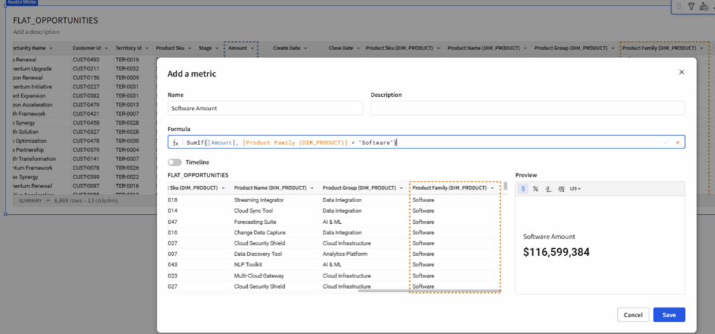
Now I can reference the “Product Family” field required for this calculation. So in order to benefit from model relationships in Sigma, relationships must be activated into a join.
Sigma also offers a different path to create a child table using an explicit join, which I typically prefer due to the clarity it creates in Sigma’s element lineage:
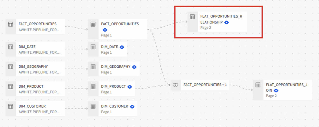
The original FLAT_OPPORTUNITIES_RELATIONSHIP table highlighted in red appears as downstream from FACT_OPPORTUNITIES, but does not indicate any relationships to the DIM_PRODUCT table it builds upon. Contrast that with the explicit join to FLAT_OPPORTUNITIES_JOIN, and we get a better visual indicator of how this was assembled.
However, explicit joins do not provide the “Data model ERD” diagram that most closely resembles Power BI’s model view. Choosing which to use in this particular case comes down to the developer’s preference, because if you want to use a dimension in a metric or visual then you will need to (at some point) activate a join either way.
Tables with activated relationships, lookup columns added and/or created from explicit joins in Sigma all create similar SQL behind the scenes: joins. And for reporting performance, joins are computationally expensive. Since Sigma pushes all compute down to the CDW and stores no data of its own, every join you add is a join executed directly in the warehouse. The more joins, the more expensive the query.
This is where the One Big Table modeling approach comes into play, and Power BI developers everywhere gasp in disbelief.
Star Schema vs. One Big Table (OBT)
So far, we have been utilizing an established star schema for our opportunities model. But as we have seen, star schemas are functionally more analytics-ready in Power BI than in Sigma. To actually operate on relationships created, we need to deliberately join facts to dimensions as an added step in a Sigma Data model.
Behind the scenes, Power BI’s DAX gets similarly translated into xmSQL that also executes joins to support dim to fact relationships. But a deeper dive into the compute engines supporting these two tools highlights that they do in fact differ in model preference:
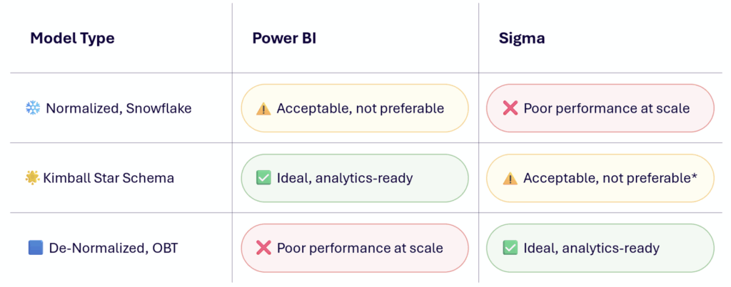
To be clear, Sigma operates great on star schemas, but performing the last-mile joins directly within a Data model is sub-optimal compared to inheriting OBTs with those joins executed upstream.
Avoiding OBTs in favor of star schemas is so engrained in Power BI development, it’s rare to even question it. But when testing differences in performance as done by the SQLBI team, it’s clear (with some nuance worth reading) that the impact is real. DAX queries involving multiple dimensions and/or moderate complexity perform much better on star schemas over pre-joined OBTs. In fact, they point out in some cases the DAX results are incorrect when applied to OBTs. The preference comes from Power BI’s VertiPaq engine and how it compresses data.
Contrast that analysis with a similar analysis done by Fivetran on CDWs, where they essentially found the opposite result: Querying OBTs with common BI patterns yields better performance than on star schemas. There was additional nuance per CDW, and a need to balance storage on large datasets that may bloat with joins executed. But ultimately the model preference is flipped.
Since Sigma sits directly on top of CDWs, best practice modeling actually looks like a materialized denormalized table to avoid the added compute from joins at query time. While Sigma can (as shown) support modeling on a star schema, doing so is only in service of creating flattened tables that could otherwise exist precomputed upstream.
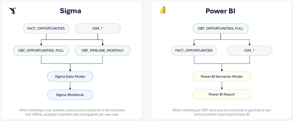
In Sigma, a star schema is a useful step towards analytics-ready tables that join facts to dimensions to support metrics and visualization.
In Power BI, a star schema is so preferable that developers will actually deconstruct a flat table out into a star schema before importing to follow best practices.
Conclusion
On the surface, both tools support similar modeling functionality. Behind the scenes, both tools convert relationships to joins at query execution. Power BI’s VertiPaq engine incidentally thrives on this approach, while Sigma’s CDW-backed compute does not.
So while many similar best-practice tenets apply, like pushing calculated columns upstream and limiting the size of tables used, the fundamental modeling best practices of these tools are not the same.
Sigma Do’s and Don’ts
There are additional differences worth covering in future blogs. Much of what is called “modeling” in Power BI translates to lineage management in Sigma. Power BI Semantic Model relationships govern filter propagation, which in Sigma requires different strategies. Ultimately the compute engines and lineage patterns in Sigma open up greater potential to operate on parallel OBTs at varying granularity to maximize performance, which looks a lot different than Power BI’s Semantic Models.
Up next: Building upon what I have covered in tool architecture and modeling, I will take a deeper dive into setting up a Workbook with controls (Power BI slicers), examining how filtering and lineage works in Sigma.