
In my previous blog post, I started with some basics of table calculations in Tableau. This post and the next are going to build on that foundation by walking through the various kinds of table calcs there are and finally discussing more advanced options for this functionality.
For each of the types of table calculations, I’ll explain what each does and apply it to an example use case, so you can see it in action. Without further ado, let’s jump in.
RUNNING Calculations
The RUNNING calculations cumulatively aggregate marks across a defined window; for example, RUNNING_SUM(SUM([Sales])) will give you the cumulative sum of sales. The value in your last mark or cell in your window should equal the total value for that window. There are other RUNNING calculations such as RUNNING_AVG or RUNNING_MIN/MAX.
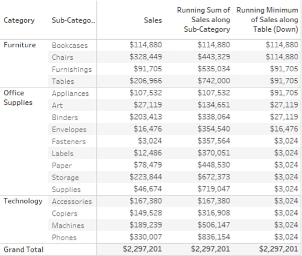
In the example, you can see two RUNNING calculations, RUNNING_SUM(SUM([Sales])) across Sub-Categories for every Category (Pane). This calculation shows cumulative sales but restarts every Category. The second calculation runs across the whole table going down and shows the RUNNING_MIN(SUM([Sales])), which effectively means that it shows the lowest Sum of Sales for the current cell and the previous ones combined, until it hits a lower value.
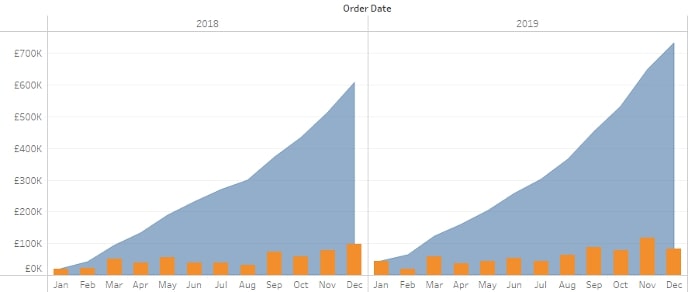
RUNNING_SUM can be used to make a nice visual combining periodic sales and total sales into one, as seen in this bar and line chart combination:
WINDOW Calculations
WINDOW calculations aggregate the data to a higher level than what’s in your view. Examples are WINDOW_SUM and WINDOW_AVG. By default, they aggregate the whole partition (window) you specify, but you can also have a moving window within the partition to create moving calculations. In this example, I added a WINDOW_SUM(SUM([Sales])) Computed Using Pane (down) to show the Category Totals:
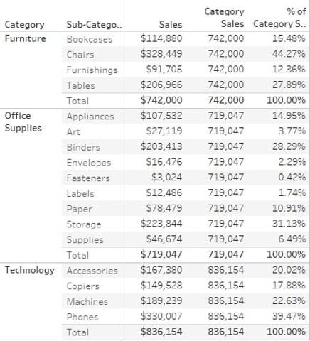
I also want to know the [Sales] by [Sub-Category] as % of the Category Totals. I can simply reuse my table calculation by calculating SUM([Sales])/WINDOW_SUM(SUM([Sales])) and ensure this is also Computed Using Pane (down).
Next up is a question from my warehouse. They want to know how long it takes to ship orders on average, and they want to track this by day. First, I create a basic calculation to measure the days between a customer placing an order and the order being shipped: DATEDIFF(‘day’,[Order Date],[Ship Date]). I then create a line chart with the day of shipping on the Column shelf and my new calculation on the Row shelf, aggregating this to average as it doesn’t make sense to sum up the days between ordering and shipping. This gives me a wild line chart, and I am not much closer to knowing how long preparing an order takes on average.
This is where the WINDOW_AVG with a moving window comes in. I add my new field, called [Days to Ship], to a new calculated field WINDOW_AVG(AVG([Days to Ship]),-6,0), where the -6 and 0 defines that I want to look back six (6) data points and include the current one to calculate my average, so I have a moving window of a week. The Compute Using is set to Table (across). In the example below, I change the -6 to a parameter instead, so I can dynamically update my window:
LOOKUP
The LOOKUP calculation enables you to take the value from a different cell and put it in the current cell. LOOKUP(SUM([Sales]),-1) essentially pushes the sales value down one cell, and this enables you to compare the current value to the previous value, for example.
In the example below, I first run a simple lookup to the previous cell across sub-category. This will leave the first cell empty for every category as there is nothing to LOOKUP and pushes the first value to the second cell. The second calculation compares the previous cell value to the current one to calculate the difference across the whole table.
LOOKUPs are useful for comparing values across the same measures. For example, they are used in the Year On Year Growth table calculations.
RANK
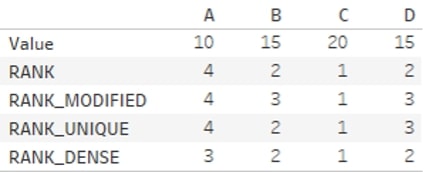
- RANK gives all values their respective competition style and rank, with duplicate values given the same higher rank (or lower rank value).
- RANK_MODIFIED works the same as RANK apart from the fact that duplicate values get the same, but lower, rank.
- RANK_DENSE works like RANK, but the missing RANK due to the duplicate value is not skipped. This means that if there are duplicate values, your highest rank is lower than the count of values being ranked.
- RANK_UNIQUE does not give duplicate values the same rank but ranks these based on the sort order, so the second appearance of the duplicate value gets the lower rank. All rank values are unique.
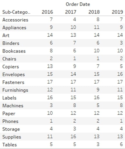
In this example, [Sub-Category] is ranked by [Sales] for every year. You can use a Quick Table Calculation to do that, however, the calculation would be RANK(SUM([Sales])). To make it ascending, starting from the lowest [Sales] [Sub-Category], the calculation would be RANK(SUM([Sales]),’asc’):
FIRST, LAST, INDEX and SIZE Calculations
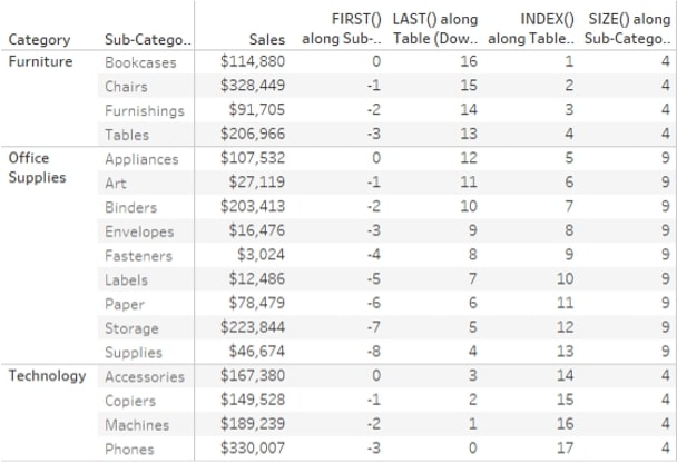
Then there is the FIRST, LAST, INDEX and SIZE calculations, which you could call cell reference calculations. FIRST returns the offset from the first cell in your partitions, LAST returns the offset from the last cell in your partition, INDEX returns the index value of the cell within the partition starting at 1, and SIZE returns the size (count of cells) in your window.
In the example below, the FIRST and SIZE calculations are across [Sub-Category], whilst the LAST and INDEX are across the whole table. FIRST and LAST can be useful in LOOKUP functions to reference the first or last value in your partition (think calculating growth). INDEX can be useful to filter to the top N records, where the standard filter does not exactly provide what you need. Since INDEX is a table calculation, it is applied after all the other filters, so there is no need to apply all other filters to context when using it to create a custom top N filter. SIZE can be useful for more complex calculations and logic; for example, when you want to only show a particular value if your window has multiple cells:
In this example, I’m using both an INDEX and a FIRST table calculation. I want to highlight the top 5 [Sub-Category] based on [Sales], as well as show [Sales] as a % of [Sales] of my top-selling [Sub-Category]. Finally, I want to be able to filter to a particular [State] without having to add this filter to the context since I might want to add an LOD, as well to show total [Sales] by [Sub-Category] regardless of the [State] filter:
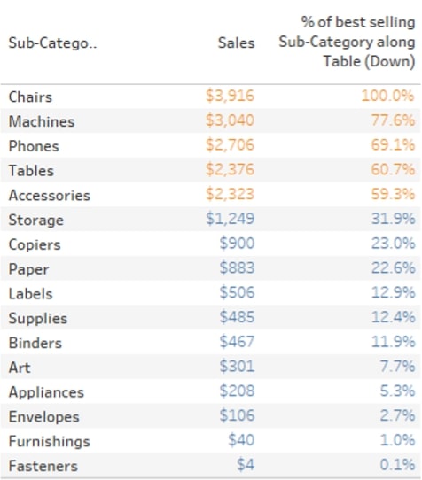
My top 5 highlighter is calculated as follows: IIF(INDEX() <= 5 , ‘Top 5’ , ‘Not top 5’). I could calculate this as a Boolean as well and change the true/false aliases. The calculation is Computed Using Table (down). Next, I want to show the % of [Sales] compared to my top [Sub-Category]. The calculation is SUM([Sales])/LOOKUP(SUM([Sales]),FIRST()). I need to ensure that my table is sorted Descending since that will ensure that the FIRST offset in my LOOKUP will always be relative to the highest-selling [Sub-Category]. You can also manually ensure that it will always LOOKUP against the highest value by using advanced table calculation options and have a custom sort order apply to the table calculation without affecting the view. More about this Specific Dimension and additional options later.
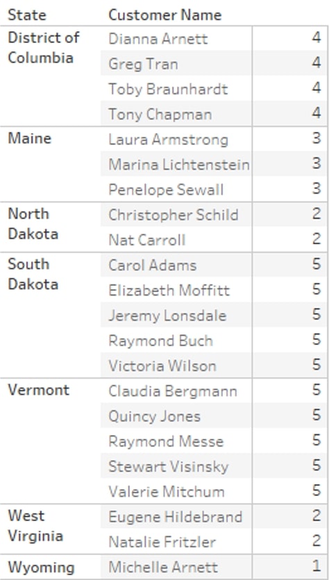
The next example is where we will use SIZE. Now, I would like a simple view showing States where we have less than five customers, and I want to show all these customers in a list. There are multiple ways to achieve this – for example, with WINDOW calculations – but we will use SIZE.
I simply create a calculation with SIZE(), and that’s it. When I put this on the Marks card and change Compute Using to Pane (down), it shows the number of records (in this case, unique Customer Names) within each pane. I move this field onto the filter shelf and filter is to At Most 5:
Finally, I’d like to have a bar chart showing my Average Order Value by Month and Year. [Sales] in its unaggregated form is a line value, so to calculate Average Order Value, I first need to aggregate the Sales to Order level and then Average that across another dimension: Month/Year of Order Date, in this case.
My calculation is going to be WINDOW_AVG(SUM([Sales])) but to ensure the Value is calculated on [Order ID] level first, I need to have this in view (if I don’t want to use an LOD). But I don’t want to show all orders in my view. One way to solve this is to only show one order for every month since the final value of my table calculation will be the same for all orders in the same month. A simple Last() = 0 on the filter shelf will sort this.
Both table calculations use Specific Dimensions for the Compute Using. This is because [Order ID] is on the Marks card and not on Rows or Columns and therefore not part of the Table or Pane:
PREVIOUS_VALUE
Finally, we have PREVIOUS_VALUE, which is a weird one. At first glance, the PREVIOUS_VALUE table calculations looks very similar to LOOKUP([Value],-1), but the big difference is that PREVIOUS_VALUE doesn’t apply to a measure you specify, like in LOOKUP, but it applies to itself.
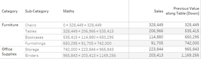
A simple example would be SUM([Sales]) + PREVIOUS_VALUE(0). This calculation would result in a running sum, as what it does is add the previous value of this calculation to the SUM([Sales]). The zero (0) argument to PREVIOUS_VALUE means that if there is no previous value, assume zero (0), but you can specify the starting value outside of your window:
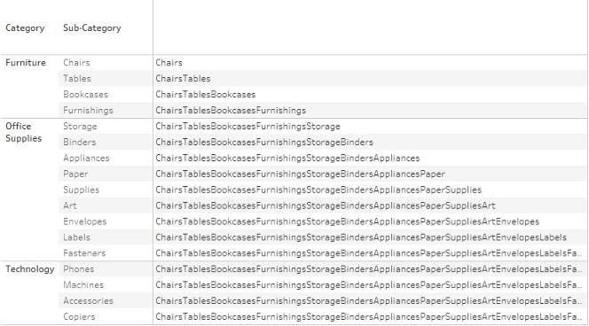
Now, I hear you thinking, “But we have RUNNING_SUM for that.” Well, yes, but there are other things we can do with PREVIOUS_VALUE such as (crazy) string calculations like PREVIOUS_VALUE(“”) + MAX([Sub-Category]), the results of which you can see below:
And you can also create compound interest calculations like this where we have a monthly interest rate, and the interest is compounded annually. The formula would be something like PREVIOUS_VALUE(ATTR([Initial Value]))*AVG((1+[Effective Monthly Interest])^12).
In the situation where you have no initial value and you deposit a small amount monthly (at the start of the month), and you compound interest monthly too, the calculation would be something like PREVIOUS_VALUE(0) +SUM([Deposit])) * (1+[Effective Monthly Interest (compounding)]).
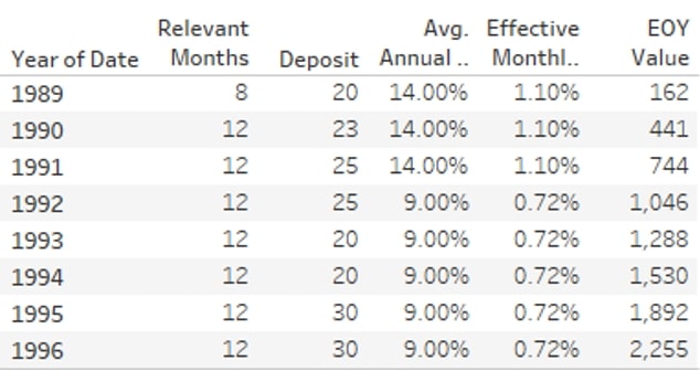
The [Effective Monthly Interest (compounding)] calculation, to account for compounding monthly instead of annually, would be SUM((1+[Annual Interest Rate])^(1/12)-1).
Next up, Advanced Options
The final installment in this series is all about the more advanced capabilities of table calculations, so be sure you check it out next!