This series takes you through various features and capabilities of Snowflake to address a wide range of business requirements, use cases and scenarios.

Conventional data warehouses of the past were designed many decades ago, built to store data in very predictable, rigid and structured formats. Back then, relational data with clearly defined schemas was the norm since data sources were smaller in volume and had less variety in terms of format. Today, with the advent of the data and cloud-computing revolution, data now originates from a wide range of sources. This now includes data coming from sensors, IoT devices and applications which store data in a non-relational, quasi-structured format.

The Rise of Semi-Structured Data

These semi-structured data formats such as JSON, XML, Avro and Parquet have become the de facto form in which this data is sent and stored from these applications because of their flexibility. However, the flexibility and expressiveness of semi-structured data also created additional layers of complexity when the data needs to be analyzed. As such, many organizations have experienced challenges to bring together both their structured and semi-structured data to generate timely business insights.

Snowflake’s Unique Superpowers

Snowflake is unique and stands out from other data warehousing platforms in the market today because it was designed from the ground up to easily load and query semi-structured data such as JSON and XML without transformation. And because an increasing amount of mission-critical data being generated today is semi-structured, Snowflake makes it easy to surface those insights to drive strategic decision-making.

Adding New Skills to Your Toolkit

This hands-on tutorial will teach you how to load JSON and XML data into Snowflake and query it with ANSI-standard SQL. If you have primarily worked with relational data models in the past, this would be a great new skill to add to your toolkit. The sample data used in this exercise features the 11 countries that comprise my home region of Southeast Asia, containing dimensions and attributes that describe each country. After going through this exercise, apart from learning how to query semi-structured data, I hope you can also get familiarized with the capital cities of each country! Our goal is to load the JSON and XML data into Snowflake to achieve the following final, end-state table:

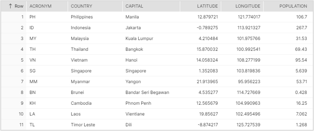
Before we get into the tutorials, download the ZIP folder here to access the SEA_SAMPLE_JSON and the SEA_SAMPLE_XML sample data files we’ll be using in this post. This folder can also be found at the bottom of the post.

Tutorial Part 1: Loading and Querying JSON Data

The screenshot below provides a read-out of the sample JSON data file:

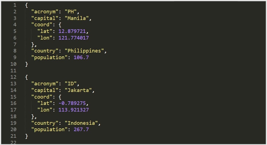
First, via the Worksheet pane in the UI, create a database called SEA_DB that will be used for storing the unstructured data in our exercise:

create database sea_db;

Set the context appropriately within the worksheet:

use role sysadmin;
use warehouse compute_wh;
use database sea_db; 
use schema public;

Create a table called SEA_JSON that will be used for loading the JSON data file. Notice that we used a special column type called VARIANT that allows Snowflake to ingest semi-structured data without having to pre-define the schema:

create table sea_json (col1 variant);

Verify that your table has been created by going to the Databases tab and then click on the SEA_DB link. You should see your newly created SEA_JSON table:

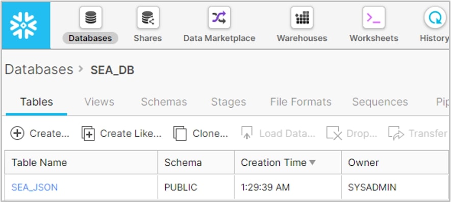
A stage is Snowflake’s way of connecting either cloud or local storage data to its platform to ingest data. It is worth mentioning that these stages can be managed by Snowflake or can point to an object storage of your choice. For the purposes of this tutorial, we will create a simple internal stage within Snowflake called SEA_STAGE:

create stage sea_stage; 
list @sea_stage;

Notice that when you ran the LIST command, nothing showed up yet. This is because we still need to import our lab data files from our local machine into the internal stage.

In this step, we will be accessing SnowSQL, Snowflake’s command-line interface tool that allows users to execute Snowflake commands from within a standard terminal. The reason why we are using SnowSQL for this step is that certain commands cannot be executed within the Snowflake worksheets environment, with the most noteworthy being the PUT command to import data into a Snowflake stage. If you are new to SnowSQL and haven’t installed it on your local machine, you can refer to this great reference written by my colleague Chris Hastie:

Using the database and warehouse we defined earlier, we can now import our two data files currently stored locally into the stage, using the PUT command. For the purposes of this tutorial, I have saved the sample data files in a folder called data in my C drive:

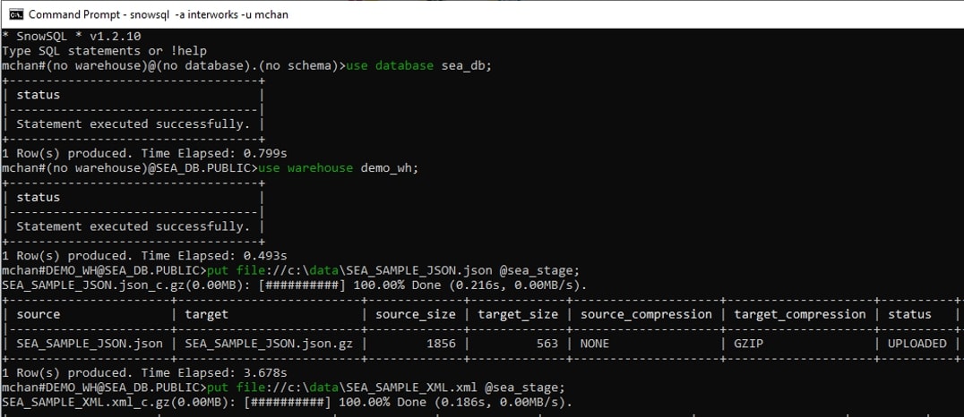
Now that the data has been imported into our internal stage, we can return to the Worksheets pane and load the JSON data from our stage into a table. Via the worksheet, run a COPY command to load the data into the SEA_TABLE we created earlier:

copy into sea_json 
from @sea_stage/SEA_SAMPLE_JSON.json
file_format = (type = json); 

Let’s run a simple SELECT query to inspect the data that was loaded. Notice how the data is still stored in its raw JSON format. Click on a row to analyze its structure:

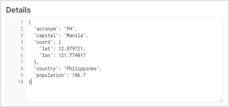
We are now at the final and most important step in this section. We will be creating a view to present our JSON data in a columnar and more readable format for end users. Notice how the SQL dot notation was used to pull out the Latitude and Longitude values from the screenshot above, which was contained in a nested hierarchy. We are also casting the fields into their desired data types using the :: notation:

create view sea_json_view as (
select
     col1:acronym::string as alpha_two_code, 
  col1:country::string as country, 
  col1:capital::string as capital,
  col1:population::float as population,
  col1:coord.lat::float as latitude,
  col1:coord.lon::float as longitude
from sea_json
);

Congratulations! You have now learned how to load and query semi-structured JSON data into Snowflake. Verify that the view has been created with a simple SELECT query:

Tutorial Part 2: Loading and Querying XML Data

This section outlines the steps needed to load and query XML data into Snowflake. The sample data file features the same data points and dimensions as in the JSON sample, so you can easily get an apples-to-apples comparison of working with the two semi-structured formats. The final output table that we shall create will also have the exact same tabular structure as in the JSON walkthrough.

Since we have already created a database and loaded the data files into our internal stage, we can now create a table and load the XML data into Snowflake:

create table sea_xml (col1 variant); 

copy into sea_xml 
from @sea_stage/SEA_SAMPLE_XML.xml
file_format = (type = XML);

Run a simple SELECT query to see how Snowflake stores the table. Notice that the entire XML file was loaded into a single row:

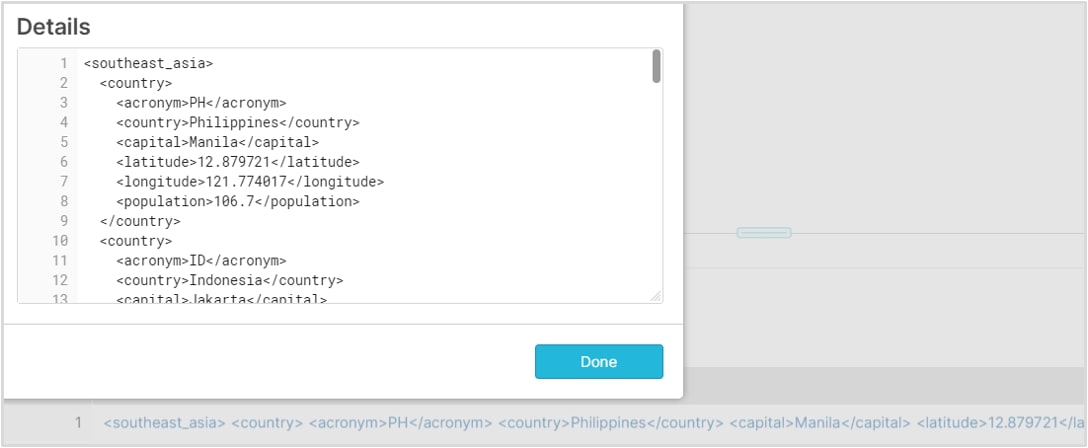
Earlier, we discussed the dot notation syntax that can be used to parse out nested JSON data. When working with XML data, a different approach must be applied. I will now introduce you to two powerful functions that form the basis for working with XML in a variant column in Snowflake. Copy the SQL script below in your worksheet, and let’s try to unpack the logic together:

select value 
from sea_xml,
lateral flatten(sea_xml.col1:"$");

FLATTEN (…) is a table function that takes a VARIANT, OBJECT or ARRAY column and converts semi-structured data into a relational structure and makes it behave as if it were a table. Running the query above should produce the result shown below. If you compare this output from our initial SELECT query, the elements have now been exploded into its own denormalized row:

Finally, as in our previous JSON example, we can save our query as a view to allow end users access to the data in a more readable manner. The final query below leverages the second important function you will need to remember when working with XML data. XMLGET (…) is a function used to extract an XML element object (more commonly known as a “tag”). It is important to note that the result of XMLGET is not the content of the tag (e.g. Singapore) but the actual tag itself (an object). To extract the content of the tag, we use the “$” operator:

create view sea_xml_view as (
select
    xmlget(value, 'acronym'):"$"::string as alpha_two_code, 
    xmlget(value, 'country'):"$"::string as country,
    xmlget(value, 'capital'):"$"::string as capital, 
    xmlget(value, 'latitude'):"$"::float as latitude,
    xmlget(value, 'longitude'):"$"::float as longitude, 
    xmlget(value, 'population'):"$"::float as population
from sea_xml, 
lateral flatten(sea_xml.col1:"$")
);

Congratulations! You have now learned how to load and query semi-structured XML data into Snowflake. Verify that the view has been created with one final SELECT query:

Next Steps

I hope you found this hands-on tutorial interesting and useful. Please feel free to message me if you have any questions! Stay on the lookout for more Hands-On blog entries in the future.