This blog post is Human-Centered Content: Written by humans for humans.

As part of my ongoing obsession with data modeling (and my day job) I have continued to dive further into Sigma Data Model functionality. In a recent exploration of feature parity between Sigma Data Models and Snowflake Semantic Views (a topic for another day), I ran into a familiar limitation on Sigma’s relationships feature. With metrics in Sigma bound strictly to their host tables, related columns can only be referenced by metrics when they are first expressed as joins.

I’ve written about this before in comparing Sigma’s modeling experience to Power BI, and the limitation here has contributed to my lukewarm feelings on the utility of Sigma relationships. Performance optimization best practices already steer away from query-time joins (i.e. the essence of a relationship) in favor of pre-materialized wide tables. With my understanding of the added limitation addressed above, the use case for building models with relationships felt pretty narrow.

Then I ran into a modeling scenario with a granular fact table containing foreign keys to dozens of dimension tables that would create a significantly wide fully-joined result. There’s a point where the performance benefit on smaller datasets could be overshadowed by the practical difficulty of navigating such a wide table. It made me wonder whether I could replicate functionality observed in a Snowflake Semantic View to lean on relationships when authoring metrics while navigating this limitation.

The obsessing yielded a discovery and solution: With a few added lineage layers, metrics can in fact reference related columns while retaining the pruned join advantage relationships provide. While this blog will cover the topic in detail, the solution is pretty simple for those familiar with the problem, so feel free to jump ahead.

I will assume some baseline knowledge on these topics, so check out these resources if you need a refresher before going further:

• Sigma’s Relationship Documentation
• Sigma’s Metric Documentation
• A prior blog: From Power BI to Sigma: Data Modeling

The Basics

The difference between using Sigma’s native joins vs. relationships is simple:

For a simple demonstration, I created two KPI elements in a Workbook with the same “Distinct Customers” metric sourced from two mirrored tables in a data model. One table uses an explicit join to a DIM_PROMOTIONS table, while the other uses a relationship to the same table. The metric in the KPI card requires nothing from the DIM_PROMOTIONS table at all, and yet the joined version contains the added SQL clause shown on the right here:

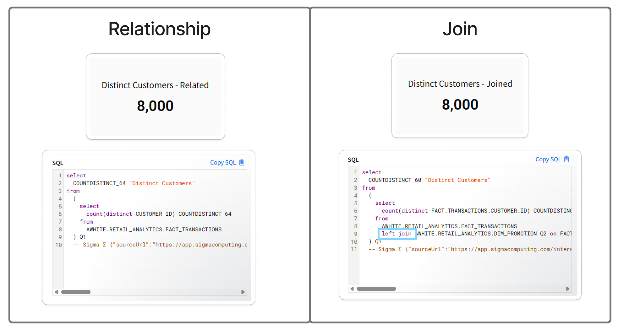
Figure 1

So when faced with modeling within Sigma, why not lean on the relationship feature to take advantage of this flexibility?

The Problem

When building Sigma Data Models with relationships, the core advantage is that downstream elements will compile SQL without the relationship joins present, until they are used. But for a metric to reference a related column, the join has to get used in its host table, seemingly nullifying the core advantage of pruning.

To see this in practice, I’ll use a model containing many related dimensions in the example below:

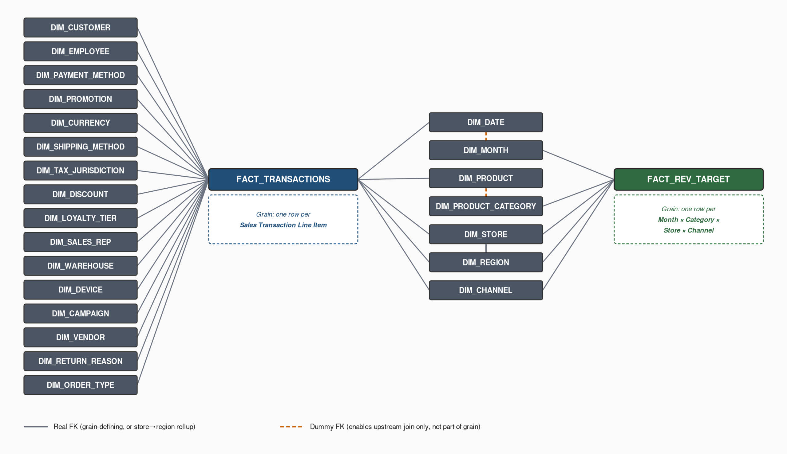
Figure 2

In a Sigma Data Model, I created table elements sourced from all these tables in Snowflake and added relationships to FACT_TRANSACTIONS in the “Modeling” tab:

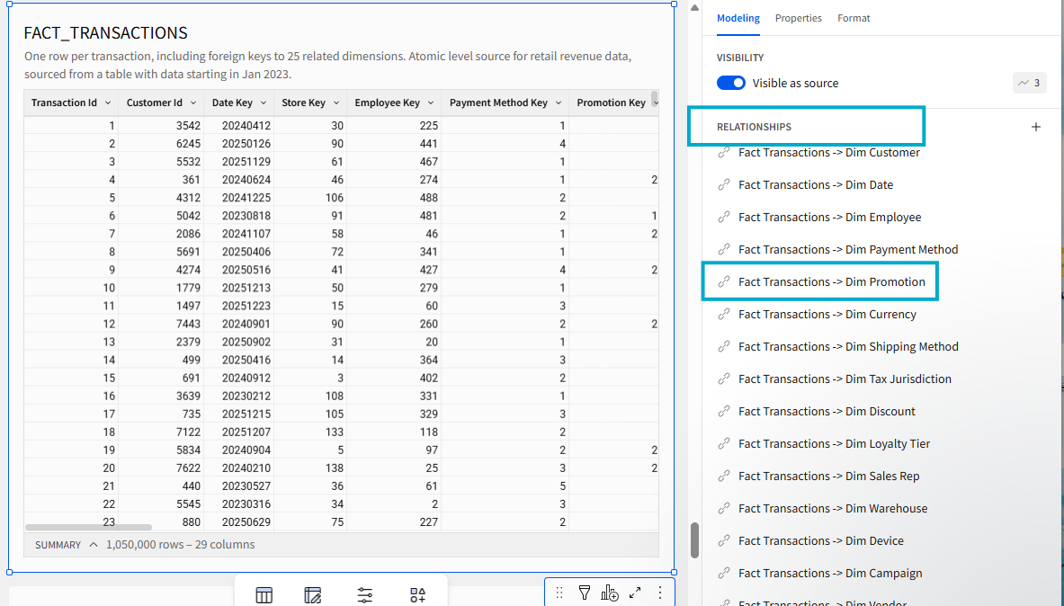
Figure 3

Next I want to add metrics, including one that measures the percentage of sales that originate from “Flash Sales” promotions.

My FACT_TRANSACTIONS table contains a Relationship to DIM_PROMOTION, which is at a per-promotion grain mapping to a “Promotion Type” category:

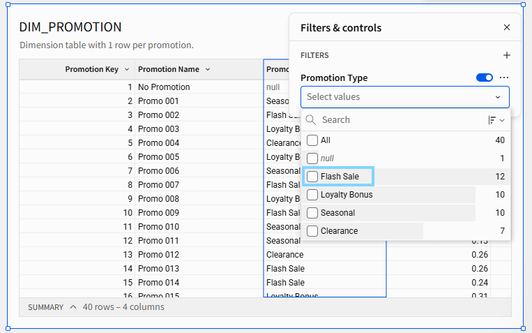
Figure 4

However, when attempting to add a metric to my FACT_TRANSACTIONS table, I only have reference options to columns already present in this table:

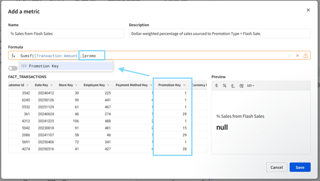
Figure 5

The closest reference I have is the “Promotion Key,” but referencing this field in the formula would be complex and not scalable with so many options to reference:

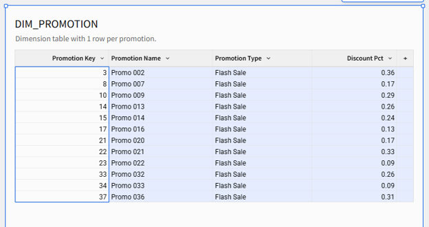
Figure 6

To reference “Promotion Type,” I need to add the column directly to the table.

Another limitation of relationships is the related columns are only available one layer below their host tables. So first, I’ll add a new lineage layer:

Figure 7

In the child table, I can now access related columns in “Available columns” and bring in the “Promotion Type” field:

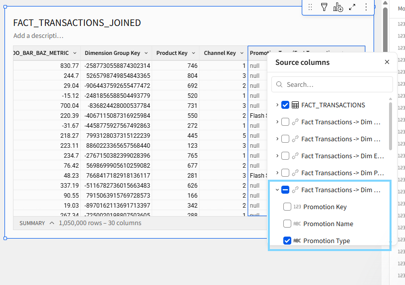
Figure 8

Doing so updates the SQL compiled to now include a left join clause to the related table:

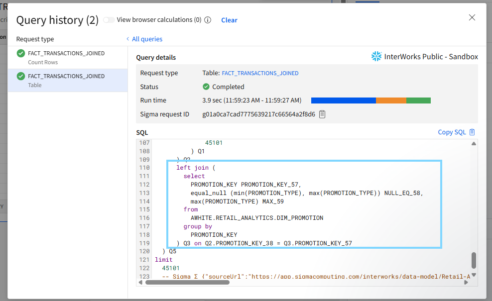
Figure 9

Now that the join is present and the column exists, I can fully author the metric referencing the “Promotion Type” here:

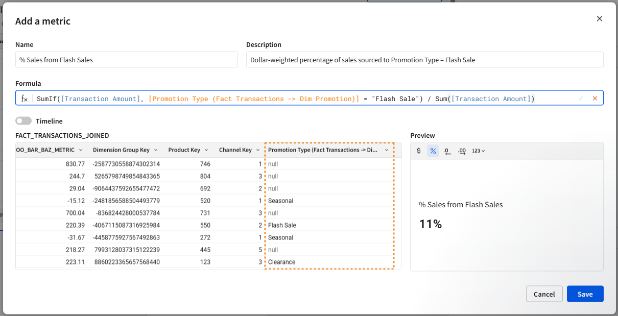
Figure 10

So to recap the above:

• My core fact table has relationships to dimension tables, but those dimensions cannot be referenced directly in metrics
• I created a child table to add the related column needed, which added a left join to the compiled SQL
• The “% Sales from Flash Sales” metric now references the joined column, sitting within a child table called FACT_TRANSACTIONS_JOINED

Here’s the problem: As it stands, every child table downstream by default now includes the left join to DIM_PROMOTIONS. And in that case, relationships and joins start to feel pretty similar.

However, through the magic of trial and error, I found that relationship join pruning works better than I thought. Going back to my simple “Distinct Customers” metric, I found that a KPI element sourced from FACT_TRANSACTIONS_JOINED did not contain the left join to DIM_PROMOTIONS, even though its source table did. So while I had to create the intermediate layer with the join expressed to author the metric, downstream elements continue to prune the join.

The Solution: A Three Layer Process

Done correctly, this problem technically solves itself. In a traditional Workbook lineage, best-practice is to land Sigma Data Model tables a base table element within the Workbook before developing downstream. From there, user-facing visuals build from the base like the sample lineage below:

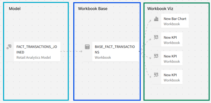
Figure 11

In this scenario, both FACT_TRANSACTIONS_JOINED from the Model and BASE_FACT_TRANSACTIONS from the Workbook will include the left join to DIM_PROMOTION based on the changes made to support the flash sale metric. However, elements in the “Workbook Viz” layer can still prune that join if they do not need it (i.e. do not use the flash sale metric nor any related columns).

This opens up broader data model use cases to support some Workbooks that require the joined fields as well as others that do not. For the latter case, as long as BASE_FACT_TRANSACTIONS is never viewed directly by sitting on a hidden page (and is not triggered as a prefetch query for Alpha Query), the only queries running will be visuals ostensibly lacking the fields triggering the join.

While that’s cool, it’s a bit confusing and disorganized for my taste, so I recommend structuring this whole process deliberately into three layers within the data model to make this frictionless downstream.

1. The Relationship Layer

The first step is creating the relationships, which was covered in Figure 3. The only added step is turning visibility off so that downstream users only connect to the finished product:

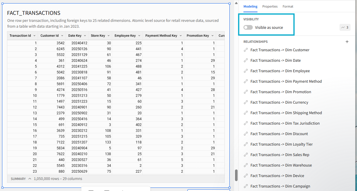
Figure 12

Importantly, no metrics get added in this layer. Metrics will be added next, and it’s best to keep them all in once place to stay organized.

2. The Metric Layer

Just as shown in Figure 7 and Figure 8, the next layer is a child table from the prior step. This allows related columns to be added to the table to author metrics like the flash sale calculation shown in Figure 10.

Once again, this layer should also have visibility turned off. Any child table connected to this layer will start with joins from columns added to support metrics, and the last layer will clean that up.

3. The Visible Layer

The last step is creating another child table, in this case sourced from FACT_TRANSACTIONS_JOINED. Since this table will be designed to be accessed downstream, I’ll give it a user-friendly name, “Sales Transactions,” and set it to visible:

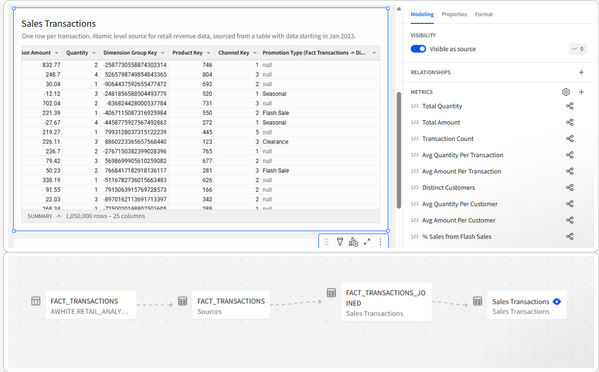
Figure 13

The next step is to clean up this table’s columns, most importantly removing the previously-added “Promotion Type.” In this case I will also remove many of the foreign keys:

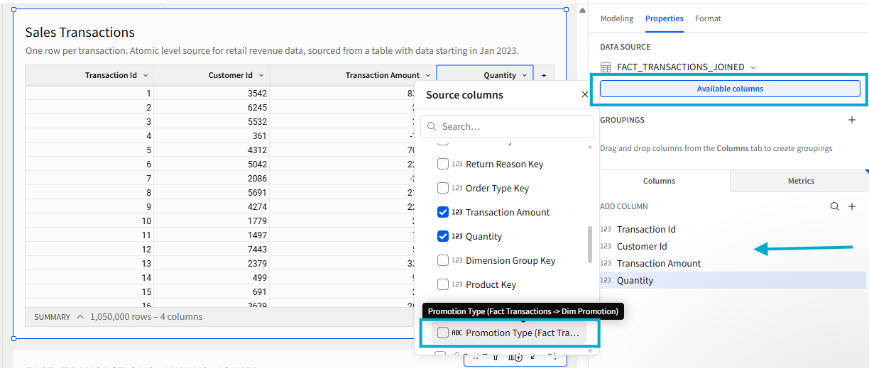
Figure 14

The SQL for “Sales Transactions” reflects the simplicity of its four constituent columns, none of which require any joins:

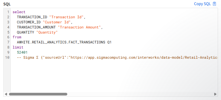
Figure 15

This is the same SQL that will run when connecting to this table from a Workbook, ensuring default behavior will prune all relationship joins until a user explicitly adds columns or metrics requiring them.

Side note: I attempted replacing this step with a Column-level Security approach instead, but the flash sale metric was no longer accessible downstream to users lacking visibility to the column.

Results in a Workbook:

With the three layers building to the “Sales Transactions” table in the data model, I can now bring this table into a Workbook to work flexibly with the relationships and metrics available:

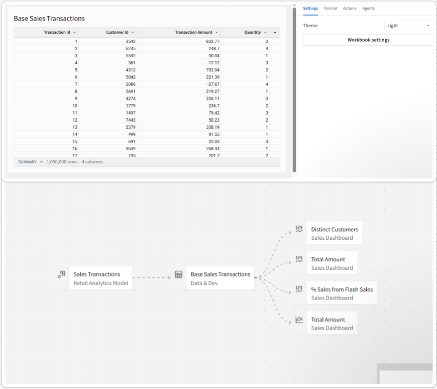
Figure 16

This lineage allows for a blend of elements that use different constellations of joins, all while sourced from a single parent element:

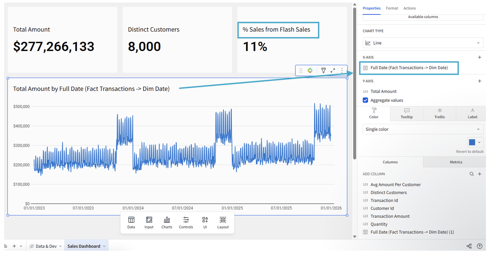
Figure 17

• The first two KPIs run simple queries with no joins
• The flash sale KPI includes the join only to DIM_PROMOTIONS (adding the metric automatically activates the join – no added step needed to add the column first)
• The line chart uses a join only to the DIM_DATE table

With these steps, we can successfully combine:

1. Metrics referencing related tables
2. Full relationship join pruning behavior

Additional Use Cases

I mentioned at the start that use cases for this functionality are narrow, but those use cases may be growing.

As Sigma developers move beyond traditional BI and into AI App development, we get confronted with the need to do more modeling within Sigma. Apps introduce more intra-Sigma modeling by design, because users are directly modifying data in real-time in the platform. I covered this in a recent blog on utilizing Alpha Query to support this development pattern, but use-cases exceeding cache memory limits require a different approach.

For an AI App leveraging larger datasets, funneling the lineage architecture through a Sigma Data Model layer would enable join flexibility through relationships as seen above. This could significantly boost performance when paired with thoughtful app design by reducing the frequency of joins needed.

Conclusion

While Sigma’s relationship functionality may not fully match Power BI’s as a preferred approach for performance optimization, overcoming the metric reference limitation puts it very close to what I have observed in Snowflake Semantic Views. The same outcome can be achieved, albeit with a few extra steps.

The standard playbook remains materializing wider tables in advance for most use-cases when performance is the top priority. But when looking for a little more flexibility, or when faced with the need to execute modeling in Sigma for whatever reason, designing Sigma Data Model lineages and visibility with these patterns opens up another set of tools for developers to utilize.