Imperative vs. Declarative Programming

There are essentially two primary approaches to coding: imperative and declarative. To put it simply, these approaches determine whether you instruct the compute engine on how to perform the program’s tasks (imperative) or what outcome you want to achieve (declarative). My colleague, Mike Oldroyd, recently shared the article A Better Alternative to Algorithms in Business Intelligence, in which he discussed the benefits of declarative programming and a desire to do so in Snowflake. Dynamic Tables, currently in public preview, represents Snowflake’s response to simplify and manage data transformation pipelines in a declarative manner. In this blog, we will delve into this exciting feature and explore its potential benefits.

Dynamic Tables

Dynamic Tables are the building blocks for creating declarative data pipelines in Snowflake. They continuously materialize the results of specified queries. With Dynamic Tables, you can streamline the data transformation process by defining the end state rather than managing a series of tasks, dependencies and scheduling. Snowflake takes care of the complex pipeline management, freeing you to focus on achieving the desired outcome without the burden of handling intricate transformation steps.

Dynamic Table syntax:

CREATE [ OR REPLACE ] DYNAMIC TABLE <name>
  TARGET_LAG = { '<num> { seconds | minutes | hours | days }' | DOWNSTREAM }
  WAREHOUSE = <warehouse_name>
  AS <query>

<name>: name of the Dynamic Table.

<warehouse_name>: the warehouse that will be used for refreshing the Dynamic Table when there is data.

<query>: specifies the query whose results the Dynamic Table should contain (declarative approach).

The TARGET_LAG parameter facilitates the automatic refresh of the Dynamic Table. The value specified represents the maximum allowed time for the Dynamic Table’s content to lag behind updates made to the base tables. It is important to highlight the “DOWNSTREAM” value for the lag, indicating that the Dynamic Table should only be refreshed when the Dynamic Tables that depend on it are also refreshed. This lag value can offer the following advantages which we will see in the example as well:

1. By using the “DOWNSTREAM” value for the lag, we can avoid the overhead of specifying individual lag times for each Dynamic Table in the pipeline. Instead, we only need to provide the lag as a number for the final table or tables in the transformation pipeline. This simplifies the configuration process and ensures that the Dynamic Tables are refreshed in a coordinated manner, optimizing the data transformation workflow.
2. While developing the pipelines, the “DOWNSTREAM” value for the lag is a valuable tool. By defining all Dynamic Tables in the pipeline with TARGET_LAG= “DOWNSTREAM”, the pipeline will not automatically refresh, giving the developer the option to invoke a manual refresh of the final table and test the pipeline. This flexibility allows for thorough testing and validation before setting the final table’s lag to the desired value.

Dynamic Tables in Snowflake offer a seamless data transformation solution for both batch and streaming use cases. You can create Dynamic Tables using regular Snowflake objects like tables and views. They also allow for complex operations like combining data, summarizing and analyzing using functions like joins, window functions and aggregates. Let’s explore a practical example to illustrate the concept in action:

Example Pipeline with Dynamic Tables

Let’s explore a transformation pipeline using a fictional scenario.  In this use case, we aim to analyze the actual versus planned sales for the franchises of a food truck brand called Tasty Bytes. To achieve this, we will work with the following base tables (standard tables).

SALES_UPDATES:  This table holds the daily order details from the food trucks of three franchises. We are focusing on data from the year 2023, and the table undergoes daily updates, which include both inserts and updates. As we commence the pipeline, the available data covers up to July 17, 2023.

TRUCK: This is a dimension table with the details of the trucks.

FRANCHISE: This is a dimension table with the details of the franchises.

SALES_TARGET: This table has the monthly planned sales for the franchises. Let’s assume that the sales number is reset every year for the franchises.

The purpose of this use case is to build a pipeline that examines the actual versus planned sales for the franchises. The data utilized for this example is sourced from An Introduction to Tasty Bytes (snowflake.com) and modified for illustrative purposes. In traditional scenarios, we typically consider options such as streams/tasks or an ELT pipeline using a third-party tool. However, in this case, we will explore how Dynamic Tables can simplify the pipeline creation process with minimal overhead.

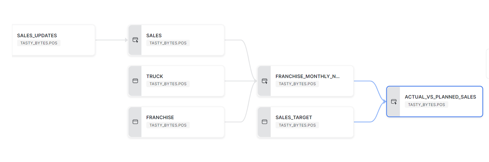
In the graph, there are three Dynamic Tables: SALES, FRANCHISE_MONTHLY_NET_SALES and ACTUAL_VS_PLANNED_SALES. We can schedule the pipeline to run once a day to incrementally refresh based on the latest records on SALES_UPDATES table.

Step 1: Dynamic Table SALES created from the SALES_UPDATES with the current records (Type 1)

CREATE OR REPLACE DYNAMIC TABLE SALES
    TARGET_LAG = DOWNSTREAM
    WAREHOUSE = DYNAMIC_WH
    AS 
    SELECT * EXCLUDE UPDATE_TS FROM SALES_UPDATES
    QUALIFY ROW_NUMBER() OVER (PARTITION BY ORDER_ID ORDER BY UPDATE_TS DESC) = 1;

The TARGET_LAG is set to downstream because we have subsequent Dynamic Tables that depend on this one. To handle scenarios where there can be multiple updates for the same order in the SALES_UPDATES table, we are using a window function with QUALIFY to filter to the most recent record per order.

Step 2:  Create a Dynamic Table to calculate the monthly sales by joining the SALES table with TRUCK and FRANCHISE tables.

CREATE OR REPLACE DYNAMIC TABLE FRANCHISE_MONTHLY_NET_SALES
    TARGET_LAG = DOWNSTREAM
    WAREHOUSE = DYNAMIC_WH
    AS
    SELECT F.FRANCHISE_ID
        ,F.FIRST_NAME || ' ' || F.LAST_NAME AS FRANCHISE_NAME
        ,YEAR(ORDER_TS) AS SALES_YEAR
        ,MONTH(ORDER_TS) AS SALES_MONTH
        ,MAX(DATE(ORDER_TS)) AS MAX_DATE
        ,SUM(ORDER_AMOUNT) AS TOTAL_MONTHLY_SALES 
    FROM SALES S JOIN TRUCK T
    ON S.TRUCK_ID =  T.TRUCK_ID
    JOIN FRANCHISE F
    ON T.FRANCHISE_ID = F.FRANCHISE_ID
    GROUP BY ALL
    ORDER BY SALES_YEAR,SALES_MONTH;

Step 3: To calculate the actual versus planned sales percentage, we can leverage the final Dynamic Table. During the development and testing phase, it is advisable to set the TARGET_LAG to “DOWNSTREAM” and manually refresh the table as needed. Once the testing phase is complete and satisfactory, we can then establish a specific lag value based on the business requirements for this final table.

CREATE OR REPLACE DYNAMIC TABLE ACTUAL_VS_PLANNED_SALES
    TARGET_LAG = DOWNSTREAM
    WAREHOUSE = DYNAMIC_WH
    AS
    SELECT 
        M.* EXCLUDE FRANCHISE_ID
        ,T.MONTHLY_SALES_TARGET AS MONTHLY_PLANNED_SALES
        ,ROUND(M.TOTAL_MONTHLY_SALES / T.MONTHLY_SALES_TARGET * 100,2) AS PERCENTAGE_SALES
    FROM FRANCHISE_MONTHLY_NET_SALES M
    JOIN SALES_TARGET T 
    USING (FRANCHISE_ID)
    ORDER BY SALES_YEAR,SALES_MONTH;

Step 4: Let’s manually refresh the pipeline.

ALTER DYNAMIC TABLE ACTUAL_VS_PLANNED_SALES REFRESH;

Invoking a manual refresh on the final Dynamic Table will automatically refresh all the upstream Dynamic Tables which it depends on.

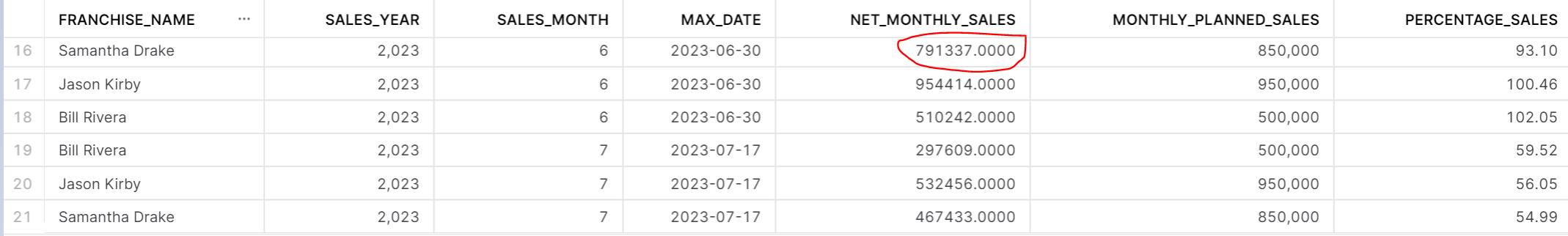
Let’s examine the contents of the final table. The screenshot below illustrates the actual versus planned sales percentage for the last two months in the dataset. Please take note of the highlighted amount as this will be altered during the incremental refresh.

Incremental Refresh

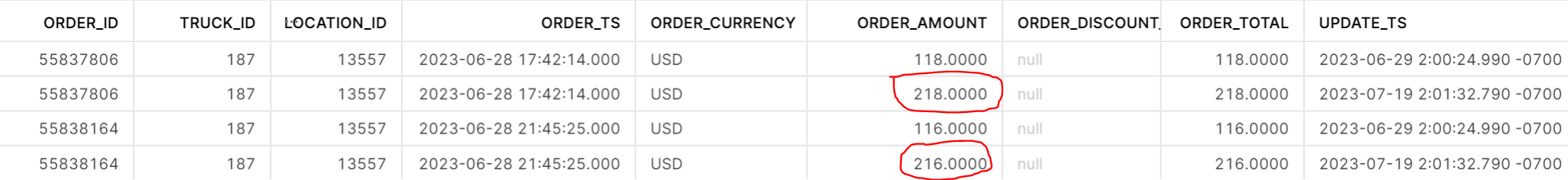
Now, let’s test the incremental refresh functionality of the Dynamic Table. The SALES_UPDATES table has been updated with daily records. In the latest batch of records, there are 3002 new records for July 18, 2023. There are two orders from June 28, 2023 with their order_amount increased by $100 each. Below are the order IDs that have had their order amounts updated in this latest batch of records (note that the SALES_UPDATES table has all historical records). We will now incorporate these changes into the Dynamic Tables to ensure it reflects the most up-to-date information.

Now that the base table has been updated with the new set of records, let’s invoke a manual refresh of the final Dynamic Table again.

ALTER DYNAMIC TABLE ACTUAL_VS_PLANNED_SALES REFRESH;

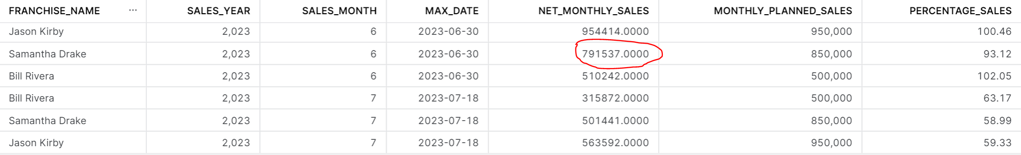
In the screenshot above, you can observe that the franchise sales data for the month of July has been updated. Additionally, there are two order IDs with a net amount increase of $200, both belonging to the same franchise Samantha Drake. The net amount increased from $791337 to $791537.

Analysing the Refresh History of Dynamic Tables for the Above Example

To gain insights into how Dynamic Tables manage the above incremental refresh, we can examine the refresh history in Snowsight. This will help us understand the approach taken by Dynamic Tables to handle the updates effectively.

SALES Table Refresh History

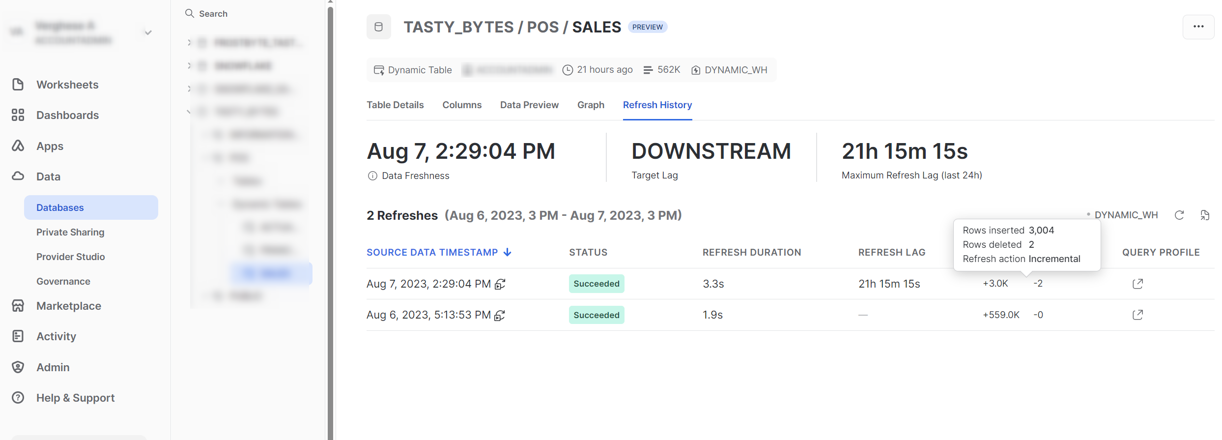
The statistics above clearly demonstrate that the Dynamic Table efficiently handled the incremental refresh according to the defined query. The table retained only one record (based on the update_ts) for the two order_ids that were updated. This smart handling by Dynamic Table highlights its effectiveness in managing incremental loads. Now, let’s proceed to explore what occurred with the remaining two aggregate tables:

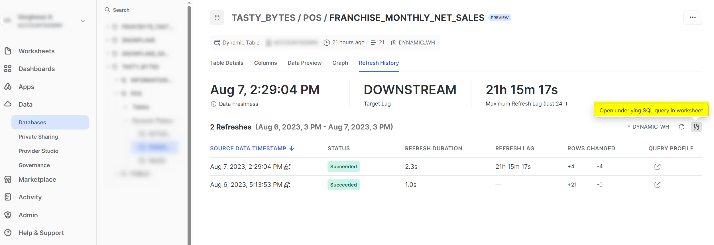
The refresh history for both “FRANCHISE_MONTHLY_NET_SALES” and “ACTUAL_VS_PLANNED_SALES” shows a similar pattern. The aggregates for the three franchises for the month of July and one of the franchises for the month of June were updated as deletes and inserts. Take note of the highlighted button in the refresh history screen of Snowsight below. This button allows you to access the underlying SQL query for the refresh history. By clicking on it, the query will open in a new worksheet, giving you the ability to customize and monitor your pipelines more effectively.

After completing the testing phase, we can set the TARGET_LAG of “ACTUAL_VS_PLANNED_SALES” to ‘1 day’ so that it is automatically refreshed on a daily basis.

ALTER DYNAMIC TABLE ACTUAL_VS_PLANNED_SALES
SET TARGET_LAG = '1 day';

The above example pipeline shows how you can build a continuous transformation pipeline with Dynamic Tables. Dynamic Tables can be also used for building slowly changing dimensions. This article from Snowflake is a good place to start.

How Does a Dynamic Table Track the Changes in the Underlying Tables?

It is beneficial to understand how Dynamic Tables handle incremental refresh by selecting only the changed data from the underlying tables. For this incremental refresh to work, change tracking should be enabled on all the underlying objects utilised by Dynamic Tables. Typically, Snowflake will automatically enable change tracking for the dependent database objects when we create a Dynamic Table. However, it is crucial to check if the role creating the Dynamic Table has sufficient privileges to enable change tracking for these objects. If there is uncertainty about the role’s privileges, it’s a good practice to verify whether change tracking is enabled for the underlying objects. Let’s examine if change tracking is enabled for the base tables in the above example:

SHOW TABLES;

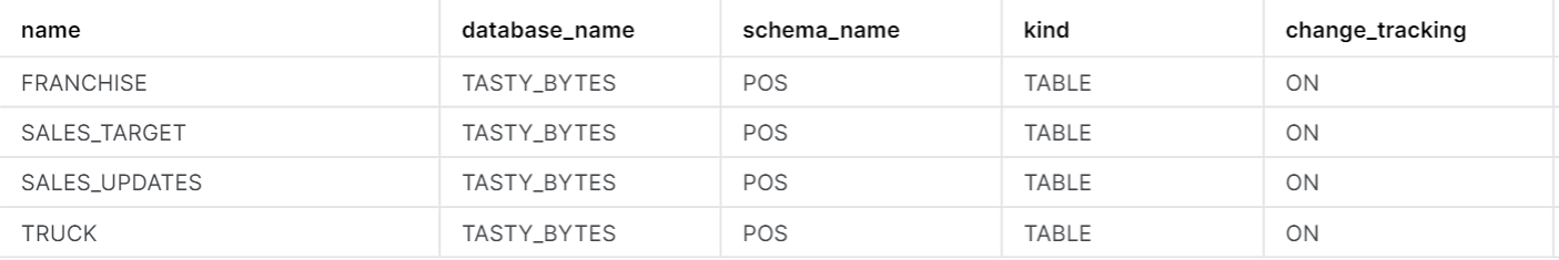
As you can see, the change tracking is enabled for all tables used within the query of the Dynamic Tables we saw in the example.

Characteristics of Dynamic Tables

1. Declarative data pipeline
2. Dynamic Tables guarantee automatic incremental data updates within the specified lag whenever feasible. However, if the underlying process cannot establish how to perform incremental refresh, such as when an unsupported expression is used in the query, it will seamlessly revert to a full refresh. Refer the Snowflake documentation for the type of queries that currently support incremental refreshes.
3. Warehouse credits are consumed for incremental refresh only if there is new data. More on this in the next section.
4. Snapshot isolation – A Dynamic Table will always ensure consistent data, as its content represents the outcome that the defining query would have produced at a specific point in the past. All Dynamic Tables in a DAG are refreshed together from synchronized snapshots, ensuring everything stays consistent throughout the process.

What Are the Costs Associated with Dynamic Table?

Dynamic Tables in Snowflake rely on a Virtual Warehouse to execute queries against the underlying base objects. This applies to both the initial load and subsequent incremental refreshes. It’s worth noting that for incremental refreshes, if no changes are detected, the Dynamic Table will not consume any virtual warehouse credits. The periodic check for incremental refreshes, performed by the cloud services compute, incurs the associated cost* for this activity. Additionally, the storage cost for Dynamic Tables follows the same model as other regular tables in Snowflake, based on a flat rate per terabyte.

*Cloud Services compute is billed by Snowflake only if its daily cost is greater that 10% of the daily warehouse cost of the account.

Strategies to Manage Dynamic Table Costs:

1. To optimize the initial sync with a Dynamic Table when dealing with a substantial volume of data, it’s advisable to use a larger warehouse for this specific task. Once the initial sync is complete, you can then alter the Dynamic Table to use a smaller warehouse for the subsequent periodic refreshes. This approach allows us to efficiently handle the large volume of data during the initial setup and then switch to a more cost-effective solution for regular updates.
2. If the incremental refresh occurs infrequently or if you do not anticipate frequent changes in data, it is advisable to enable auto-suspension for the warehouse used for the Dynamic Table. Snowflake will not resume the warehouse if no changes are detected during the periodic check. If the data changes are expected frequently or there is a near real-time ingestion requirement, it is more practical to keep the warehouse running, as there is a 60-second minimum billing each time the warehouse starts. The decision to leave the warehouse running should be based on the anticipated change frequency to ensure cost-effectiveness and efficiency.

Some Data Engineering Considerations:

1. Setting the keyword “downstream” in the lag will make sure that the dependent Dynamic Tables of a downstream Dynamic Table will refresh based on its refresh needs. Snowflake will elegantly handle the synchronization.
2. The manual refresh of the Dynamic Table uses the warehouse defined in the Dynamic Table even if your session is using a different warehouse. It is therefore advisable to only execute manual refreshes using XS warehouses, as they will not be performing the refresh themselves and you do not want to burn credits by having a larger warehouse execute this command. Another option would be to alter the lag of your table to 1 minute, wait for a refresh to begin, then alter the lag back to what it was previously.
3. Data pipelines can be constructed using a combination of streams, tasks, merges and Dynamic Tables.
4. Streams can be built on top of Dynamic Tables. A stream based on a Dynamic Table works like any other stream.
5. The decision about Dynamic Table latency should be guided by the business requirements and a good balance between cost and performance.
6. Alerts and notifications can be leveraged to notify the user for any pipeline errors or warnings. Explore the example below for a better understanding.

An Example of Snowflake Alert to Notify Users of Dynamic Table Refresh Errors

The Snowflake alerts and notifications feature provides valuable observability into your data workloads. For more in-depth information, you can refer to this blog post. Let’s take a look at an example of how to create an alert that monitors a frequently refreshed Dynamic Table pipeline and notifies you in case of any refresh failures. This alert will be triggered every hour to examine DYNAMIC_TABLE_REFRESH_HISTORY if the most recent refresh encountered any errors. This proactive approach will help you stay informed about the health of your pipelines and ensure timely action is taken in case of any issues.

CREATE OR REPLACE ALERT ALERT_DYNAMIC_TABLE_REFRESH_ERRORS
WAREHOUSE = DYNAMIC_WH
SCHEDULE = 'USING CRON 0 * * * * UTC'
IF ( EXISTS
(
WITH MOST_RECENT_RUNS AS (
      SELECT
          *
      FROM TABLE(
          INFORMATION_SCHEMA.DYNAMIC_TABLE_REFRESH_HISTORY(RESULT_LIMIT => 10000)
        )
      WHERE STATE NOT IN ('SCHEDULED','EXECUTING')
      QUALIFY ROW_NUMBER() OVER (PARTITION BY DATABASE_NAME, SCHEMA_NAME, NAME order by DATA_TIMESTAMP desc) = 1
    )
SELECT 1
FROM MOST_RECENT_RUNS
WHERE STATE NOT IN ('SUCCEEDED')
)
)
THEN CALL SYSTEM$SEND_EMAIL (
'EMAIL_NOTIFICATION_INTEGRATION',
'<email recipients>',
'ALERT:Error identified during dynamic table refresh',
'An error has been identified during the automated refresh for one or more dynamic tables. View the details of this error by querying the DYNAMIC_TABLE_REFRESH_HISTORY table function or checking the Snowsight refresh history view. Note that this alert runs every hour, so the same error may be alerted multiple times until the table is refreshed successfully.'
);

Current Limitations

The underlying query for a dynamic table currently cannot include the following constructs:

• Materialized view, external tables, shared tables, streams or stored procedure
• External functions
• Views on Dynamic Tables
• Non-deterministic functions except those mentioned here

Snowflake is continually evolving and gradually adding support for more complex SQL features in Dynamic Tables. Therefore, it’s advisable to stay updated with the Snowflake documentation to stay informed about the supported features.

What New Features Can We Expect in Future?

1. Latency less than 1 minute – as of now the minimum latency is one minute. However, Snowflake has already indicated in certain summit sessions that they are in the process of reducing this latency to just seconds. This advancement holds the potential to enable near real-time data ingestion and immediate utilization of transformed data, especially when combined with Snowpipe streaming.
2. We are optimistic that Snowflake will eventually introduce serverless capabilities for Dynamic Table load and refresh. This advancement would eliminate the overhead associated with managing the virtual warehouse, resulting in a more streamlined and cost-effective solution for data load and refresh operations.

Summary

Dynamic Tables are a game-changer in Snowflake, making data transformations easier than ever. With their simplified, declarative approach, you can let Snowflake handle the pipeline complexity. Ready to harness the power of Dynamic Tables? Step up your data engineering game with Snowflake today!