
Picture this: You are trying to build a sales dashboard in Tableau Desktop to show your boss how great you are. But hey, there is one issue: The data you have is currently in a structure not suitable for Tableau Desktop. You need to crosstab or pivot the data on several measures and dimensions. The data source can’t be changed or manipulated at the source level, as it’s on SQL Server or several other departments need the data in that format as it is for other reports.
Sound Familiar? Well, you will be happy to hear that this is the situation that Tableau Prep is made for. No longer will you need to bring in the same data source multiple times and combine the workbook on a tricky blend.
Tableau Prep allows a user to build a workflow that transforms data step by step until it is suitable for Tableau Desktop. This blog post shows how pivoting and joining can clean up data to make it suitable for Tableau. It will show how to simply and easily split data into different Branches, pivot the data on different columns and join these back together.
The Data
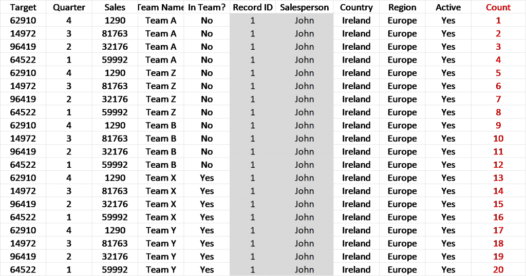
Table 1 below shows the sample data that Is being used. It holds quarterly sales and sales targets for each Salesperson, as well as if they are part of different Teams. The data also holds information on geographical characteristics, as well as if the salesperson is active.
There are four key sections of this data that are necessary for shaping the data for Tableau.
-
Unique Identifiers
This relates to the column/columns that give the data a unique value. In this case, the Unique Identifiers are Record ID and Salesperson. These can be seen in the Red box in the screenshot below. In this case, using only one of the columns would act as a unique identifier; however, in bigger data sets, more than one column might be necessary. Both will be used in this case.
-
Sales by Quarter
This located in the Blue box. This is the first of the three pivots that will take place in the workflow.
-
Sales Target
This data is in the Green box. This is the second of the three pivots that will take place in the workflow.
-
Team Data
This data is in the Orange box below. This is information on what Team each Salesperson is allocated to. It will be the final pivot of the workflow.
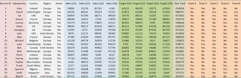
Table 1
Workflow Setup
The first step is to connect Tableau Prep to the data source. This is very similar to how it is done in Tableau Desktop. Once the data has been selected, Tableau Prep shows an overview of the data that has been brought in.
In this section, it is possible to edit your data by renaming Field Names, deselecting unwanted columns and filtering data values. This is done via interaction with the metadata interface (located in the Red box).
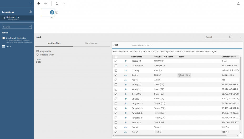
Figure 1
The other change made to the data is filtering by the Active column. This is because I only want active salespersons. This is done by hovering over the cell which intersects the Active field name and the Filter column (see the Blue box in Figure 1). Once this is done, a prompt will appear to filter the data. This brings the user to a calculation box like in Tableau Desktop. In this calculation only, Boolean calculations can be utilised. The answer can be only true or false. The calculation will only keep the data that is true. The calculation will be the following: The data is going to be edited by getting rid of the column Year Total, as the data will not be required once pivoted.
[Active]=’Yes’
The next step is to split out the workflow into a number of “branches” so it is possible to pivot on the three measures required. To do this, click on the plus (+) on the interface page. This gives the user several options of what they would like to do with the data. See Figure 2a below.
To make the first branch of the workflow, click on Add Step, as this will allow users to make changes to the data. Once you have done this, go back to the same plus (+) and click Add Branch (Figure 2b). This will allow the user to transform the data separately from the original branch. Repeat this step twice more until there are four branches (Figure 2c).
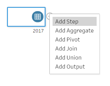
Figure 2a |
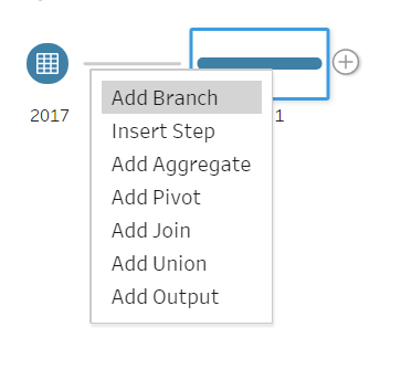
Figure 2b |
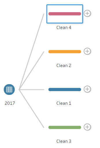
Figure 2c |
The reason for the four branches is that three are for the pivoting of the data while the fourth is for the rest of the data that is not being pivoted. Although it is possible to do this with three branches, it is best practice to use a fourth, as it prevents confusion by keeping the pivot simple with only relevant data to that pivot.
It is possible to name the branches by double-clicking on the text below each step. The renaming will be the following:
- Clean 4 – Rest of Data
- Clean 2 – Team Pivot
- Clean 1 – Sales Pivot
- Clean 3 – Targets Pivot
In each of the branches, the columns Record ID and Salesperson will be kept, as these are the unique identifiers and will be used to re-join the data post pivoting.
To remove fields that are not required for each branch, the user must click on the step that has been renamed, e.g. Team Pivot. When clicked, a tab will pop up below. This will give a breakdown of the data in each of the columns. In this interface, it is possible to remove the fields that are not needed in this part of the workflow. This is done by right-clicking the field and click Remove Field or highlight fields that are unwanted and click Remove Field above the column headers.
As you remove the fields, you will see a description of the actions in the changes tab (see Green box in Figure 3). These can be deleted to undo specific changes.
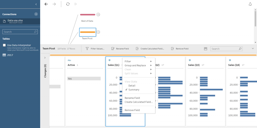
Figure 3
The data columns that are required for each branch are as seen below:
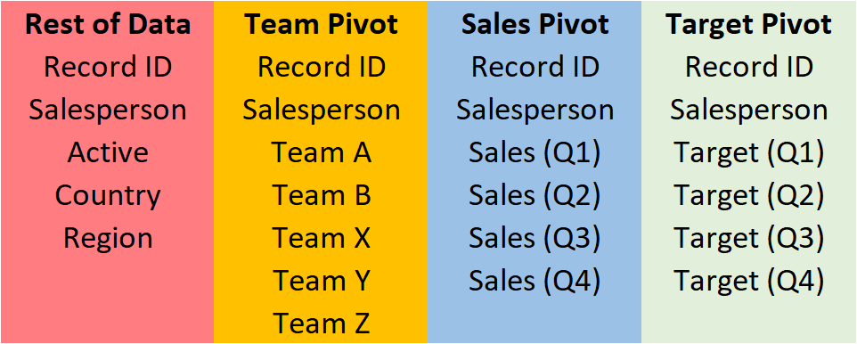
Figure 4
Once the unwanted fields have been removed from the workflow. We will begin to pivot the data.
Data Pivoting
The first Pivot will be the Team Data. This is the team that the salesperson is part of. To do this, click on the plus (+) on the step named Team Data and select Pivot. This will add a new step within the interface, as seen in the image below.
The interface within the Red box shows the current fields in the data branch. The Blue box contains the interface where the pivot is created. The values that you wish to be pivoted can be dragged from the Red box to the prompt Drop fields here. When this is done, the fields that have not been selected will be kept in the Red box section. There is an option automatically rename pivoted fields and names by checking the box above this section of the interface.
The Green box shows what the data output would be. This is a good check to ensure that you are pivoting correctly. This can be interacted with; it is possible to split, remove and rename columns here.
A way to ensure that you are pivoting correctly is to check the number of rows in the top-left corner of the interface. The desired number of rows after the pivot is the number of original rows, multiplied by the number of columns pivoted. In this case, there 17 rows before the pivot and five columns being pivoted. Therefore, the required output is 85 rows.
Instructions
- Drag the five Team fields into the Pivot1Values box (Figure 4a-b)
- Rename “Pivot1 Values” to “In Team?” (Figure 4c)
- Rename “Pivot1 Names” to Team (Figure 4c)
Step 1
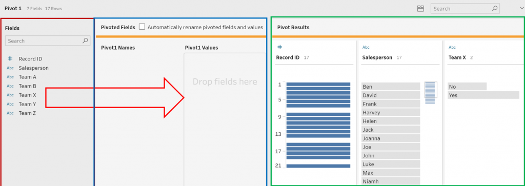
Figure 4a
Step 2
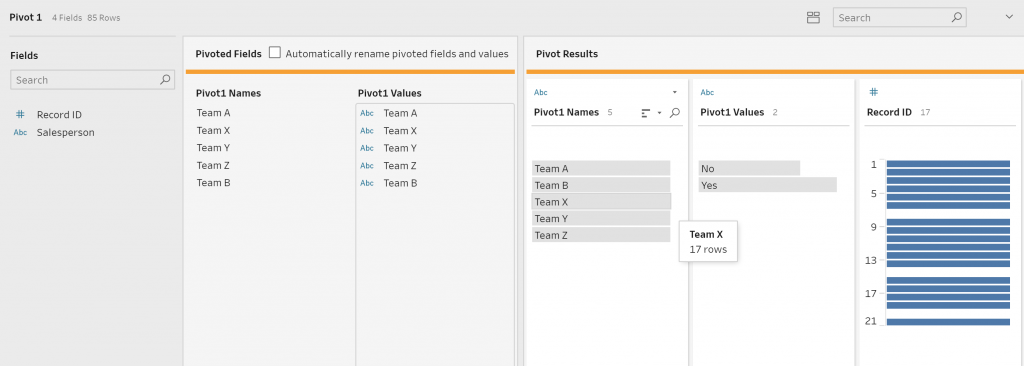
Figure 4b
Step 3
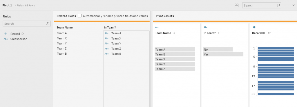
Figure 4c
Join Pivot to Rest of Data
The next section is to combine the newly pivoted team data to the branch that contains the rest of our data. To do this, click on the step that was renamed Rest of Data and choose the option Add Join. Here we can join the two branches together based on the Unique Identifiers.
To Join the data, click and drag the pivoted data onto the join, a prompt to ‘Add’ will tab out from the Join step. Hover over the add and the data will act to join the data together. The data will error at first as there is no data being joined yet. (Figure 5a, b, c)
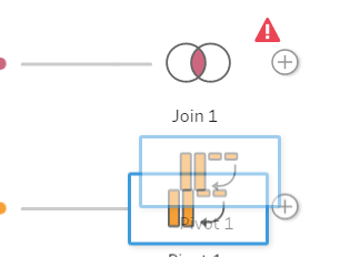
Figure 5a |
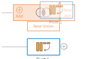
Figure 5b |
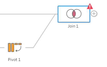
Figure 5c |
An interface will pop up from the bottom of the screen with options how to join the data. There are options to pick what fields to join on, what type of join is required (Inner Join, Outer Join, etc.). A summary of what has being joined or being mismatched is located here, as well as a recommendation on what fields to join on (Figure 6a).
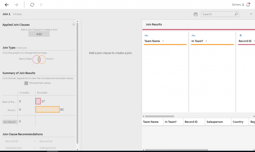
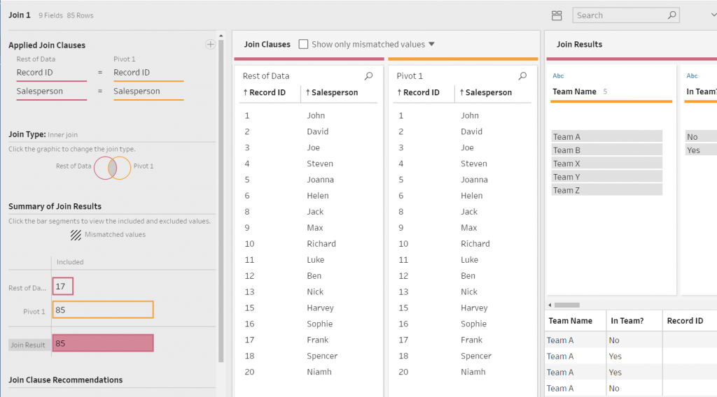
To create a join, click the Add box found under Applied Join Clauses and select the Field Names for each Data Branch to join. In this case, it is Record ID and Salesperson. An inner join will be executed in this instance. Once there has been a join, the interface will convey what values from the joining fields have matched. There is also an ability to view what values have not matched.
The right-hand of the interface contains the breakdown of the data, similarly to previous steps; however, the fields are colour-coded based on what data branch they are sourced from.
The next process is to clean this join my removing duplicate fields. Repeat the steps completed after adding the branches to the workflow. Any duplicate fields have the suffix “-1.” It is easy to search for this and remove these.
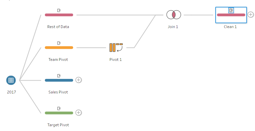
At this point, the workflow should convey something like Figure 7.
Quarterly Sales and Target Pivot
Next is pivoting of the quarterly sales data. The pivot will be a similar process to the Team Pivot. For the Sales Pivot, the Quarterly Sales fields will be dragged into the Pivot1 Values box. Except in this case, instead of renaming the fields, we will add a new step to the workflow. This is because in the Pivot1 Names field, the values read the word “Sales,” plus the quarter; the quarter value is the only value required.
In this new step, we will split the Pivot1 Name field by right-clicking the column, hover over Split Values, and click Automatic Split. (Figure 8a) This derives a new column, Pivot1 Names – Split 1, which contains values 1, 2, 3, 4 referring to the quarter. (Figure 8b) This is to be renamed “Quarter.” The original Pivot1 Names can be removed, as it is no longer relevant. Pivot 1 Values can be renamed “Sales” (Figure 8c).
Repeat these steps for the Target Data:
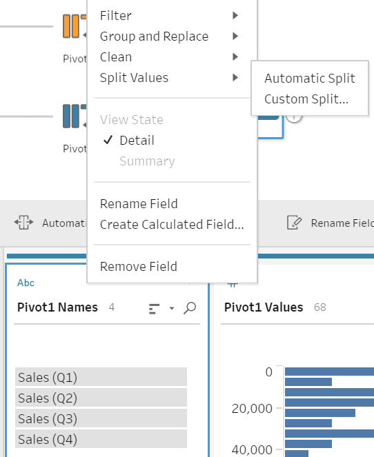
Figure 8a |
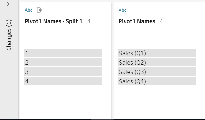
Figure 8b |
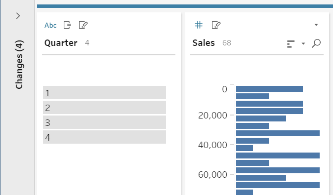
Figure 8c |
Joining Quarterly Data
Now that we have pivoted both the Target and Sales Data, we can join these branches together. Similarly to the previous join, we will create a Join step on the Sales branch, Add Target to the join. The only difference is that Quarter will also be joined on to one another as well as Record ID and Salesperson. A step will be added after the join to remove any duplicated fields.
NOTE: When looking at metrics over time, it makes sense to join on the same time record if possible, as this allows more comparisons going forward. Instead of quarterly data, the data could have been yearly or monthly.
At this point, Figure 9 should look similar to your workflow. So far, the three streams of data have been pivoted on the required fields. Duplicated fields have been removed, the Team Branch has been joined to the rest of the data, and Sales and Target data have been joined together.
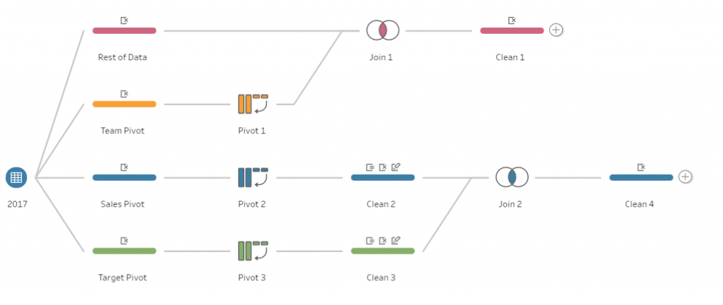
Figure 9
The next step is to join the combined quarterly data to the branch combining the Team Data and the rest of the data. This is a repeat of the first join. The join will be on Record ID and Salesperson. This is the final join of the workflow. Now at this point, the data is in a shape that is coherent in Tableau. The final step to clean the data fully will be to remove the duplicated fields created from the join
A way to double check that your pivots and joined have been correctly implemented is counting the number of rows a unique identifier is in. The count should equal the number of fields pivoted by one another (see Table 2). For example, in this case, the Record ID / Salesperson should be seen 20 times (5 teams X 4 quarters).
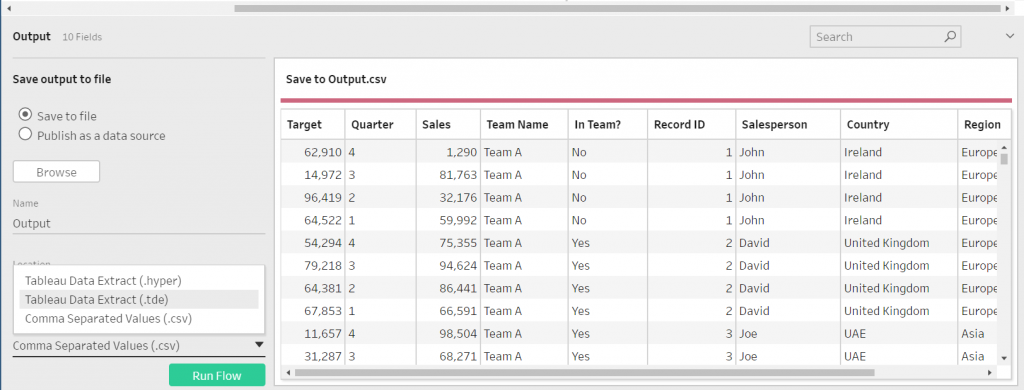
Outputting Data
Outputting data is very simple. Click on the plus (+) on the step. Once the data has been fully cleansed, select Add Output. This will bring up an interface that prompts where to save the output, the name of the output and type of file the output is (tde, hyper or csv). To create the output, the workflow is run by clicking the Run Flow button at the bottom of the interface (Figure 10).
Saving the Workflow
Similarly, to Tableau Desktop, workflows in Tableau Prep can be either saved as packaged or non-packaged. The packaged workflow (.tflx) will contain the data with the workflow. The non-package workflow (.tfl) will just contain the workflow, but no data will be contained.
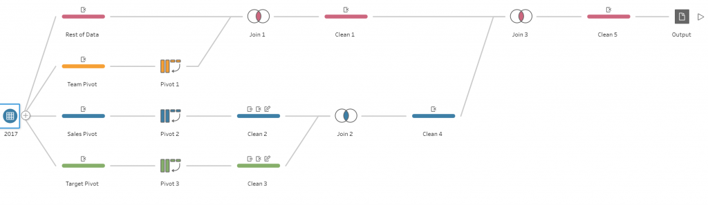
For reference, the full workflow should look like Figure 11.
A tip for running workflows, once you have created an output but are still developing the workflow, is to make a copy of the output. Without this, the workflow will error if it is being used in a Tableau Workbook. Each time you make changes to the workflow in the development stage, copy and paste the output.
You can download the full Tableau Prep workflow I used here.