Joins—they are happening everywhere. That’s actually a cool tagline! And it’s definitely true. I haven’t encountered a data warehouse, a data lake or a BI tool that didn’t include some sort of join somewhere.  

But I also know there are a lot of explanations about joins out there … like thousands, and certainly a few really good ones. So why add another? Well, in many of those thousands of resources, I find good explanations but no visuals. Others have great illustrations, but no explanation. Many have good explanations and illustrations but use a bad example no one can relate to. Then there are a few articles that are very well done but targeted at coders only. (One of my favorites is probably the one from C.L. Moffat on Visual Representation of SQL Joins in 2009 that makes it really easy to get into joins.) 

Now, this article here in front of you is for everyone. If you are completely new to joins, this article is for you. If you are already comfortable with joins, this might be a refresher for you. If you do joins while you are sleeping and dream of Venn diagrams instead of sheep, you might stay and give me some feedback on the article. (Also, there is a reason why you landed here, I presume. 😊 ) 

So, let’s talk a bit about joins, why we need them, what they are and how they work. 

Let’s Start with the Why 

Why would we join tables? Well, the reason is pretty simple: We might not have one but two tables of data in front of us. (Or a whole lot of them.) And although the data is in two different places, we know it belongs together, and we would really like to unify it into one table rather than two. 

We could, for example, have a list of our colleagues, classmates, friends, family or whatever social group you prefer with all their names and birthdays. You also have another table, again, with all these people in it, but this time with their favorite hobby next to their names. These two tables could come in extremely handy if we were looking for birthday present ideas:

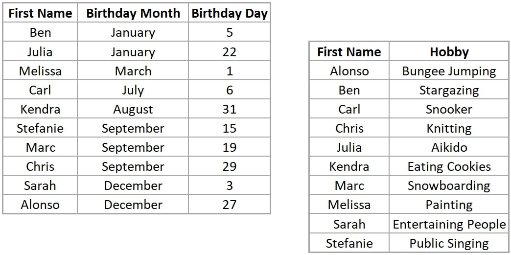
But it would be even more convenient if we had names, birthdays and hobbies in the same table: 

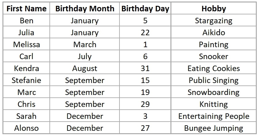
Better, right? We don’t have to look for a name twice as the sorting in the two tables is different.  

Now, What Is a Join? 

In Excel, we could work with a VLOOKUP to get the right cells. But we are talking SQL or Tableau or other BI, analytics or data-shaping tools here, which are not cell-based like Excel but table-based. 

Joining tables means merging them in such a way that columns are appended. We have a table on the left (birthday list) and another table on the right (hobby list). What we want to do is build a new table out of the two that has all the data we need, so we don’t have to use the two separate tables anymore. 

To make that work, we cannot just put both tables next to each other. If we did, the data lines of both tables wouldn’t match unless we have that rare case where both tables have the same granularity, size and are ordered exactly the same. We need to force these two tables together so that the First Names match up. This is what joining does: 

We select a specific field—a key—that appears in both tables and is an identifier (in our example, the First Name from the birthday table and the First Name from the hobby table), that tells which name in the right table belongs to which name in the left table. Once we do that, all rows from the right table get attached to the rows of the left table wherever the First Names are matching up. 

Now you may ask the question: What happens when there are rows that don’t have a match? And what happens when I have First Names with several matches in the hobby table? Happens all the time, right? Well, joins are pretty straightforward. Their basic rule is that they try to find matches for the key fields. Each match equals a row in our final product. But I’ll explain by answering a few of the frequent questions I get in trainings, combined with our birthday present idea table. 

What if I Have Several or No Matches in a Table? 

Joins look for matches. In your case, a record in the left table might have a few record matches in the right table. Just remember: each match produces a row. Let’s have a look at our example, and let’s also say that we know more than one of Kendra’s hobbies: 

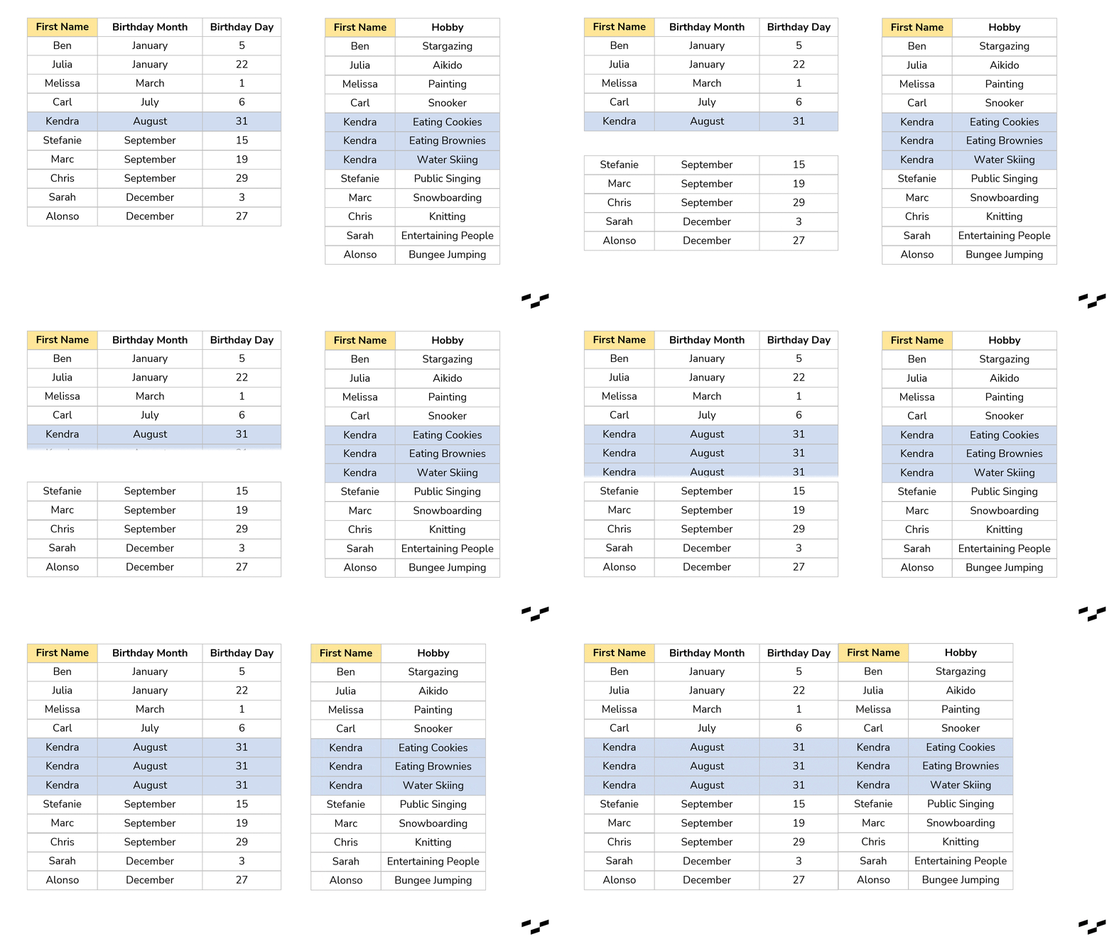
Notice that rows in our left table get duplicated. Kendra appears now three times, like in the right table. The join found three matches between left Kendra and right Kendra, so there are three records. 

Right away, this is also the biggest downside joins have. They are extremely helpful in shaping and manipulating our data, but when the granularities in both tables are different, we get duplicated rows. To get the number of unique names, we now have to use a distinct count instead of a simple row count. If we had another field in the left table that gives us the amount we are willing to spend on a birthday gift, for example, this number would be duplicated as well (lucky Kendra!). So be mindful of that. 

This is when we have more than one match per record. What if we have less than one, so no matches? 

This question leads us to NULLs and to join variations. First, every time we join two tables and there are non-matching records, joins produce NULL values. Some tools just show empty cells or rows instead of NULLs. In our example, let’s say, we have lost Chris and Carl. Or maybe we don’t know them well enough and have no hobby data. Also, there is Matt, who we know likes wood carving, but we have no idea when his birthday is. 

The join (in this case, a full outer join) would produce empty cells in both tables: 

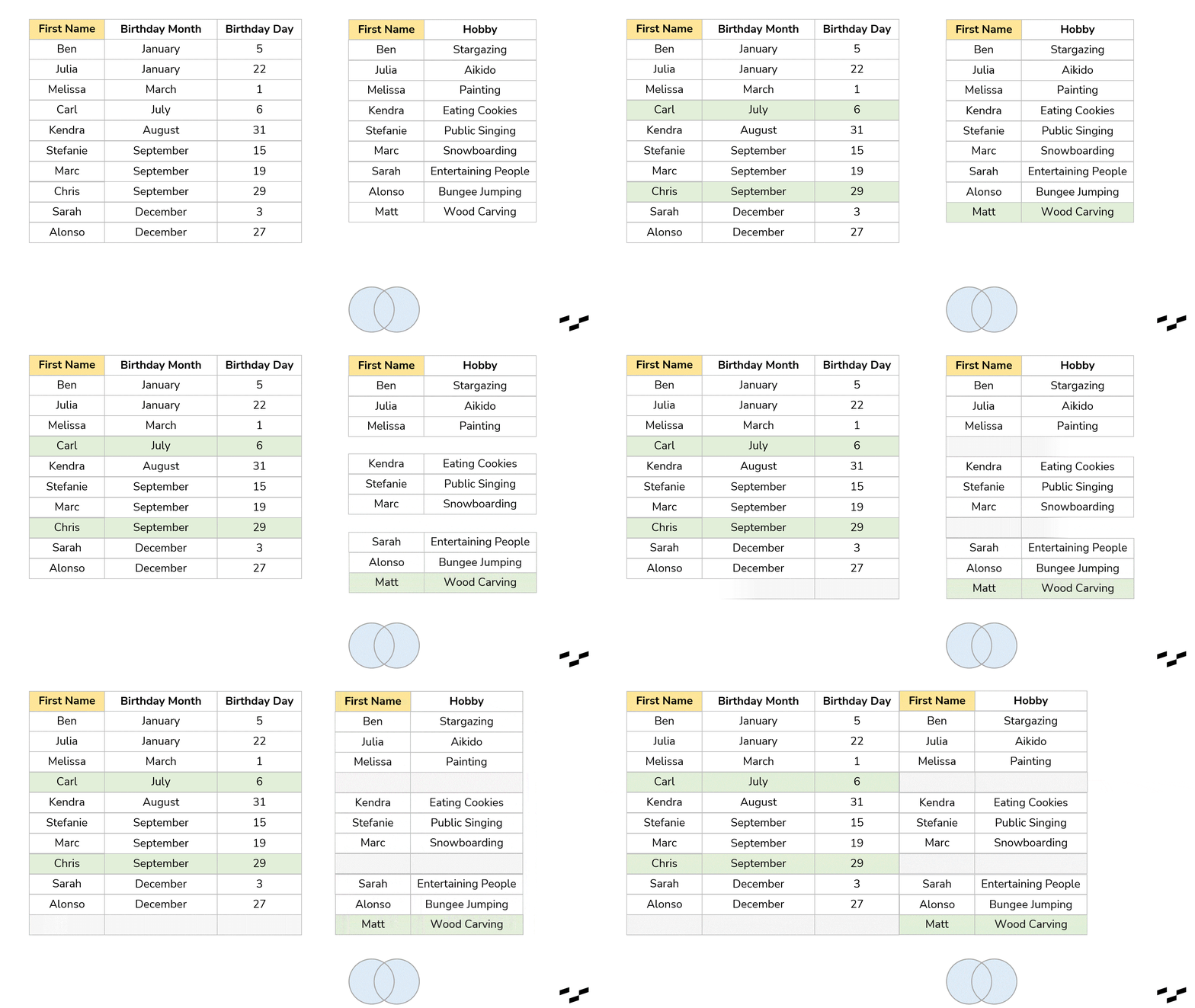
Sometimes, that is exactly what we want. Maybe we don’t have data for all records in both tables, but we still want to enrich our final table with the data we have.  

Nonetheless, sometimes we want something different. My birthday present table, for example, won’t make sense if I don’t know the hobbies of my friends. So, the names in there without a hobby are not relevant to me at all. (I will still congratulate them, but here we are talking presents.) And the other way around: If I know what they like but don’t know their birthday (Matt), the records won’t matter as well. We can tell the join to only build the rows for which we actually have matches. 

Join Variations 

Enter the join variations. There are quite a few of them. The Venn diagram is the most common icon for joins, and how this diagram is filled is telling us what kind of join it is:

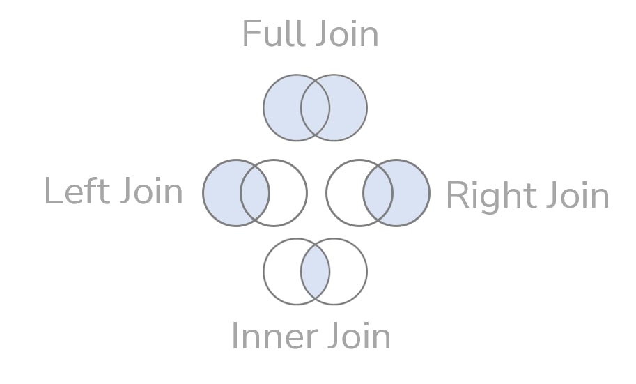
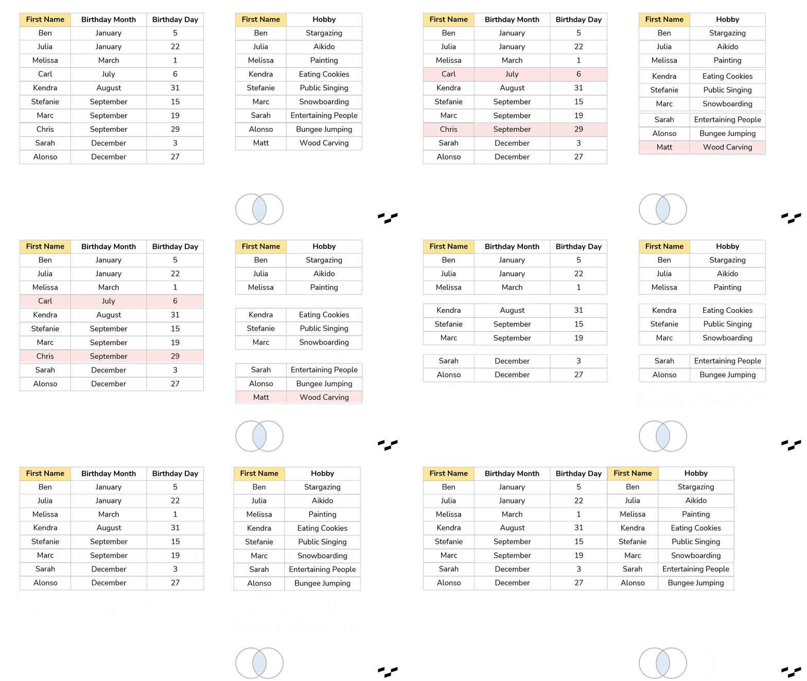
What we have done above with our birthday tables is a full (outer) join. It indicates that it takes all the rows from the left table and all the rows from the right table. It joins the rows that have a match; all other rows produce NULLs in the other tables.  

If we want a birthday present table that only shows records that have a match in both tables, we would need the inner join. This one discards every record in both tables for which the join doesn’t find a match. What is left builds our result: 

Of course, there are more. Let’s see what a left join does with the exact same table: 

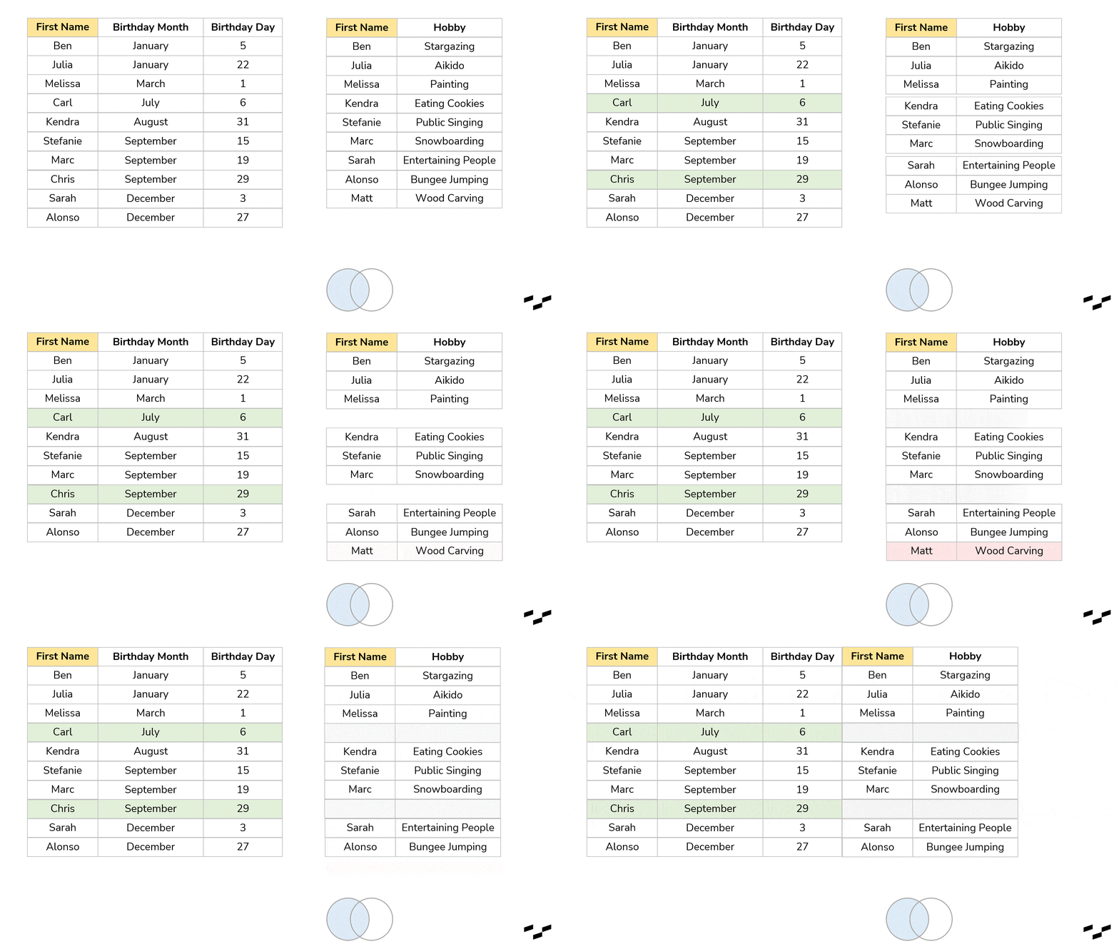
You may notice that all records from the left table are part of our result. In a left join, all rows from the left table will always be there, while we only get rows from the right table that have a match in the left one. Goodbye, Matt. Records from the left that don’t have a match in the right table (Carl and Chris) get NULL values. The right join will work exactly like this but the other way round. The right table will be the dominant one of which all the records are retained: 

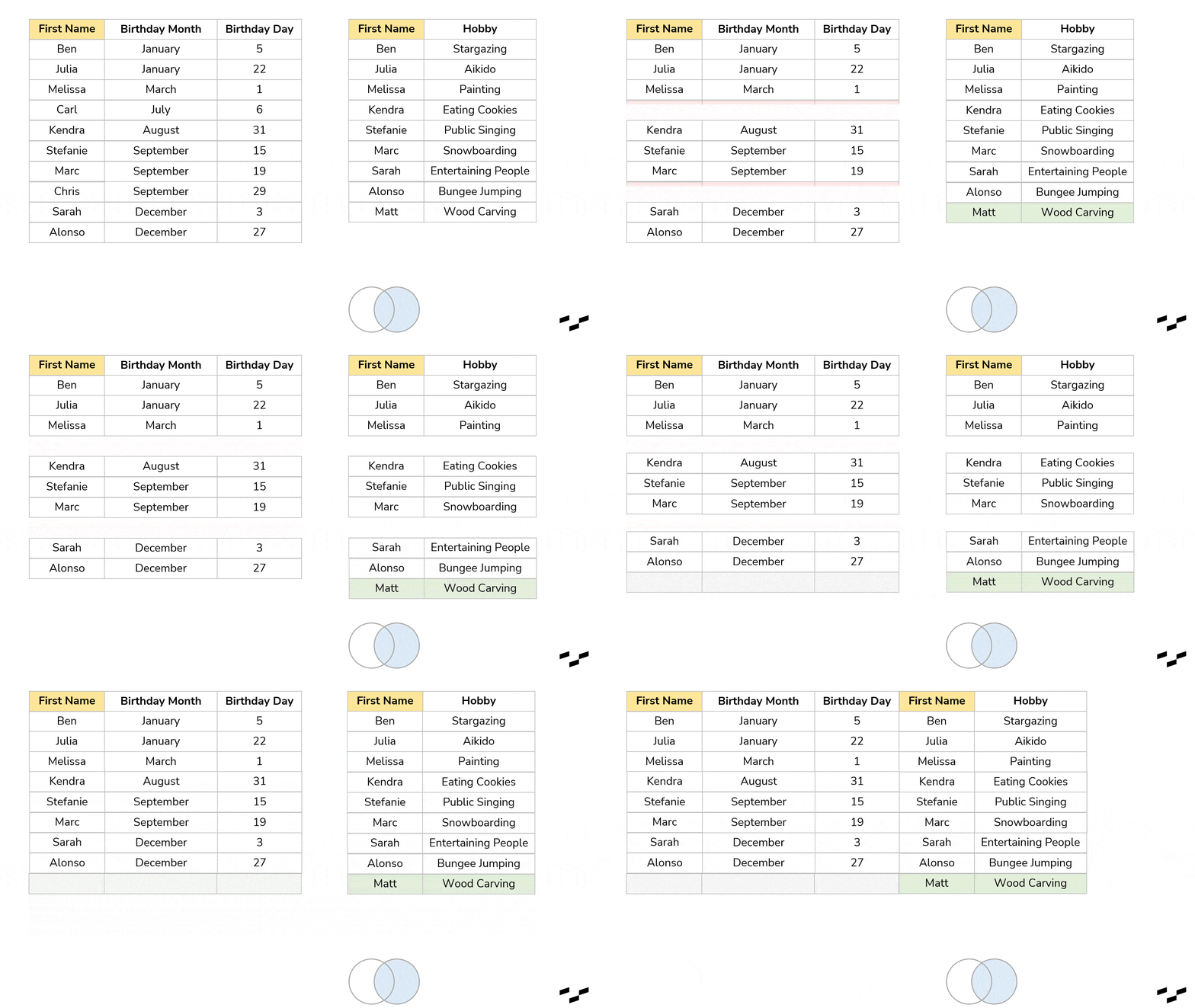
These are certainly the most frequent join types. Also, for those of you who work in or with Tableau: these four are the only join types that Tableau supports when building a data source (without the usage of custom SQL queries). 

There are a few more that we can build in SQL, but as they are the exact counterparts of the ones we have seen already, I won’t show examples:

You might notice that the left excluding join is exactly the part that is left for good in the usual right join, vice versa for the right excluding and left joins, and yet again for the full excluding and inner joins. 

• A left excluding join in our birthday example would give us all the rows that don’t have a match in the right table, which would be Carl and Chris. 
• A right excluding join would give us all the rows that don’t have a match in the left table, which would be Matt only. 
• A full excluding join then would give us everything, that doesn’t have a match, being Carl, Chris and Matt. 

The three excluding joins are sometimes also called anti-joins, like in left anti-join. Especially the Microsoft universe with Power BI and PowerQuery uses those quite eagerly. (By the way, they also have another word for a join. They call it merge.) 

The Cross-Join 

This one is special. Even its Venn diagram is different. Cross-joins have several other names by which they are known: Cartesian joins, Cartesian products and 1-on-1 joins. 

Cross-joins are used to multiply our rows. Okay, that may be too simple. They are used to get each and every possible combination of rows of both tables. To show that with our birthday example, I have to crop our tables; otherwise, we would have about 100 rows in here. So, let’s go with three names only—Ben, Julia and Melissa:

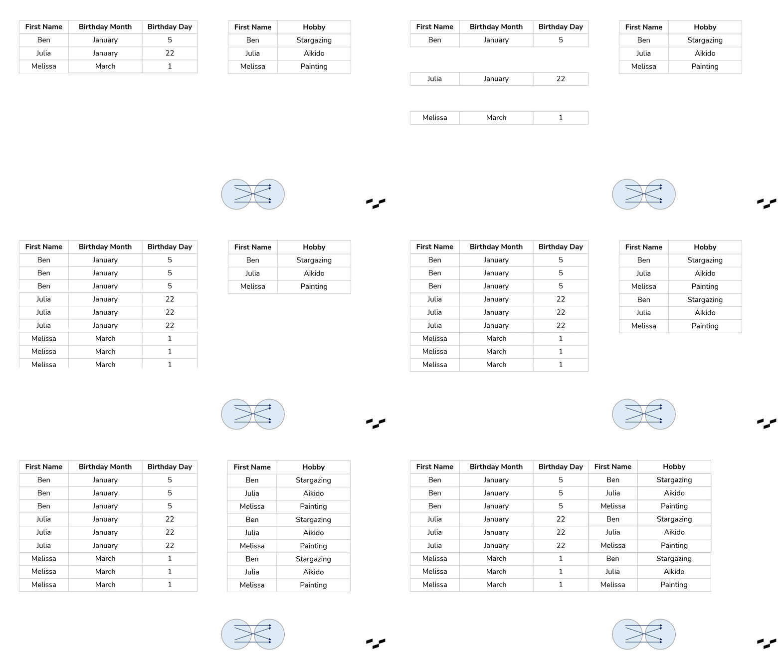
You may consider cross-joins as joins without any real mapping at all. All a cross-join does is map every row from the left table with every row from the right table. For our birthday lists, that doesn’t make any sense, of course. In six of the resulting nine rows, we have wrong name matches. 

Why should we ever use cross-joins? Well, to understand this, let me remind you that we can filter our data down later on. Meaning, when we have joined or modeled our data, in 99.9% of all cases, we aren’t done yet. With cross-joins, we almost never are. With that being said, imagine that we have two tables we want to bring together, but there is not a single field we could use as a key field or mapping field. We find that quite often in HR tables, for example, where we have:

• Table A: a list of employees and their hours, they have to work each day,  
• Table B: a calendar, already curated, to see bank holidays or company-wide events.  

Now the business question might be: How many hours did all of my employees work last year? To get the answer, we can just cross-join employees and calendar dates and sum up all the hours in our new and very long table. 

Another use case might be a performance test. We can cross-join a table to itself, which squares its row count, going from like 10,000 rows to 100,000,000 rows. That may happen when we work with sample data, but we’d need to test the system for the production data later on. 

By the way, the name 1-on-1 join comes from one way the cross-join is built in SQL or other tools like Tableau: two new fields are created or defined, one in the left table and one in the right table. All rows contain the number 1 for both fields. Then, it’s these two fields that are mapped to each other: 1-on-1. 

A Few Last Notes 

You will encounter the phrase full outer join or left outer join quite often in the programming world. There is no difference between a full join and a full outer join. Adding the word outer makes it a bit more obvious that we don’t do an inner join, but there is nothing more to it; no technical difference.  

Also, I have been asked once: If every usual join we see has its counterpart, what about the full join? Yes, I did not draw this scenario. Technically, it would be two empty circles, but data-wise that would just mean no data. And as such, we are allowed to neglect that. There is no nothing join or empty join. Yeah, I’ve actually heard both before.

And there you have it! A crash course into the world of joining tables.