What do you do when a request can’t be solved by traditional reporting tools, and adding new tables or views to your database can take weeks? 

Situation 

A new manager joins the group. While you’re presenting your workbook, she wants to see things a little differently. Instead of top 10 sales by state, she wants to compare one state’s sales against another state’s sales. She gives you an hour to get it done before she hops on a plane to Zurich.

In order to handle our new manager’s request, we want to simulate the results of a CROSS JOIN (Cartesian product). Through this, we can define a relationship of every Column A entry to every column B entry. See the example below:

EXAMPLE: Cartesian product.

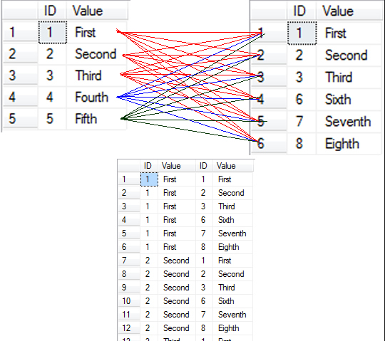
This result set can be quite large when dealing with even a few hundred records because 1000 customers by 50 states suddenly becomes 50000 rows! Because we don’t want a huge result set, we’re going to want to filter by only the relevant information in our analysis.  

These situations are typically handled with a little custom SQL, but what if you don’t know SQL (or even what to Google)? Worst of all, what if your SQL guy is spending the day at ComicCon?

What to do now?  

Enter the Blend  

When bringing additional data sources into your workbook, our mantra is “join if you can; blend if you must.” Sadly, people take this advice to mean that they should avoid blends instead of looking for the circumstances where blends can really advance your analysis.

One of my teammates has already tackled this intra-dimensional comparison and delivered a custom SQL answer (Business Questions and Data Structures). Today we’re going to explore the same challenge via blending, and allow anyone with a basic understanding of blending and data sources to produce some powerful results.

NoSQL “cross join” overview via blending:

• Connect to data source
• Duplicate data source
• Build out view in primary data source
• To help organize our efforts, we will make our calculated fields in our primary data source 
• Break the link field so we don’t blend on a single state; we will maintain a higher level of aggregation or grouping
• Use a filter to identify the state that has our attention (show me only what I want to see)

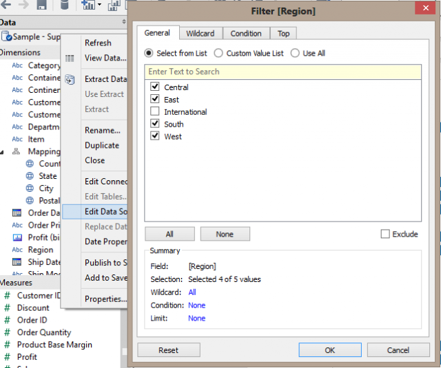
Step 1: Open Tableau and Connect to Your Data

NOTE: In order to match the original solution (see above) and because I want to filter out international data prior to aggregating my sales data, I’m filtering out the international business from the sample Superstore Data via a data source filter. To create the filter, right click Data Source, select Edit Data Source Filters and add your filter – e.g. Region.

Step 2: Duplicate Your Data Source

Right click your data source and select “Duplicate.”

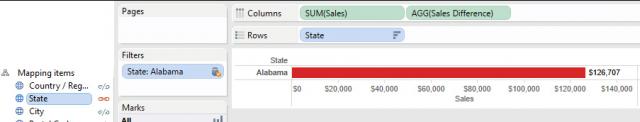
This blend works like a cross-join since the results will be the same for every state in the primary view.

STANDARD BLEND (on linking field) – only the selected state in the filter is blended.

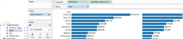
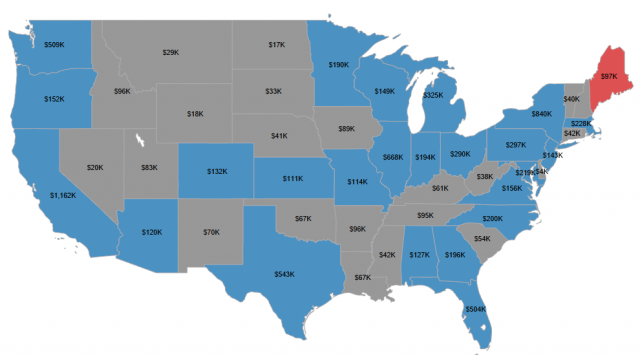
Blending with no linking field – all states from the primary data source are shown.

 

NOTE: In order to achieve this blend, from your secondary data source, click the red link icon that is automatically activated on State (break the link). We don’t want to actually blend data on the state level.

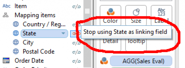
As seen above, if we keep the link activated on State, we’ll only bring in data from our selected state. This is not our desired behavior. We need the unlinked blend, otherwise the post-aggregate join (blend) would filter out the rows in the primary source that match the state (then we’re back where we started).

See the following example:

Our State and Sales data appear in this form in Excel:  

State	Sales
Maine	97000
Vermont	40000
Utah	83000

When we filter on Maine with a linking field activated, our query will return the following:

Maine – 97000

In Tableau, it will appear like this:

Blend Active (linking field on): Selected State = Maine (

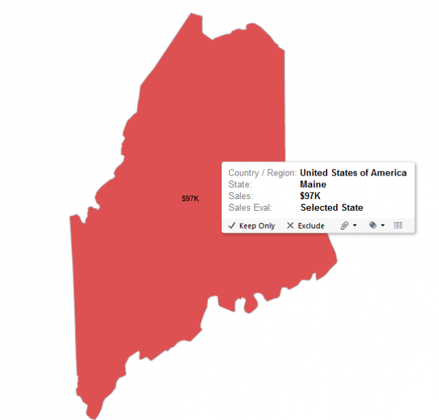
Without a linking field, we receive the sales information for all the states.

Blend Inactive (linking field off) : Selected State = Maine

Step 3:  Build Your Initial View, Establish Your Primary Data Source

Drag Sales to columns.

Drag State to rows.

Sort State by Sales descending.

Step 4: Create Two Calculated Fields

Sales Difference:

From our primary data source, select Analysis then Create Calculated Field.

Take the absolute value of the difference between the Sales field from the secondary data source.

Note: The field is pre-aggregated and so is the Sales field from our primary data source.

ABS(SUM([Sample – Superstore – English (Extract) (copy)].[Sales]) – SUM([Sales]))

Sales Evaluation:

Use our filter to identify our selected state and states with lower and higher sales:

IF MIN([State]) == (ATTR([Sample – Superstore – English (Extract) (copy)].[State])) THEN  “Selected State”

ELSEIF SUM([Sales]) > SUM([Sample – Superstore – English (Extract) (copy)].[Sales]) then “Greater”

ELSE “LESS”

END

Step 5: Finish Out Your View

Drag Sales Difference to Columns (next to Sales).

From our secondary data source, drag State to the Filters shelf. Right click and select Show Quick Filter.

Note: Your view should disappear until you select a choice from the filter.

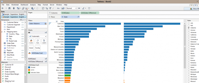
Step 6: Format Your Workbook and Pat Yourself on the Back

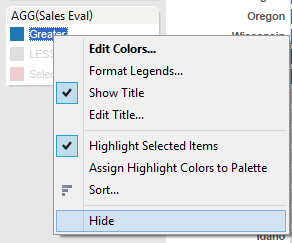
Pro Tip: To show only states greater than or less than our selected state, select Greater from the legend then select Hide.  

What’s Going on Under the Hood?

By unlinking on State we send two queries out: one to the primary datasource, which brings back all the states. The other query is sent to the secondary datasource, returning only the state we care about via the filter on the secondary data source.

This scenario actually gives us a performance edge over a standard cross join because of the a la carte comparisons we can perform with our quick filter without bringing over data we’re not interested in.

Because of size and organization of data, your mileage may vary with real world datasets. When performing this example with your data, my recommendation would be to optimize your extracts by rolling up aggregation to a monthly or quarterly level and hide unneeded columns.

There you have it! In the time it would take to locate your SQL guy or to Google how to write this query, you handled the challenge. Now you’re probably wondering about the wonderful chocolate your boss is going to bring back for you from Zurich.

Good luck in your future blending!