In Microsoft Excel there are a handful of ways to style a table or apply shading to alternate rows. In Microsoft Excel 2010 and Microsoft Excel 2007, after you have highlighted what cells you would like to apply the the styling, under the Home tab, one can click on Format as Table and click on what styling you would like.

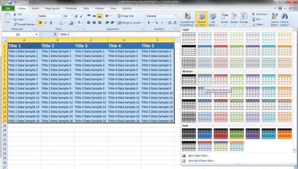
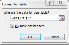
My data set lies within columns A to E and rows 1 through 17. Since I highlighted my cells before I clicked Format as Table, my data for my table was already inserted in my range of data.

But lets say I want to highlight every 5th row because every 5th row of data is important. In this case, row 5, row 10, row 15, and row 20 Note: I added a few rows into my next example to round up to 20 rows of data and added a column called ROW # for this example.

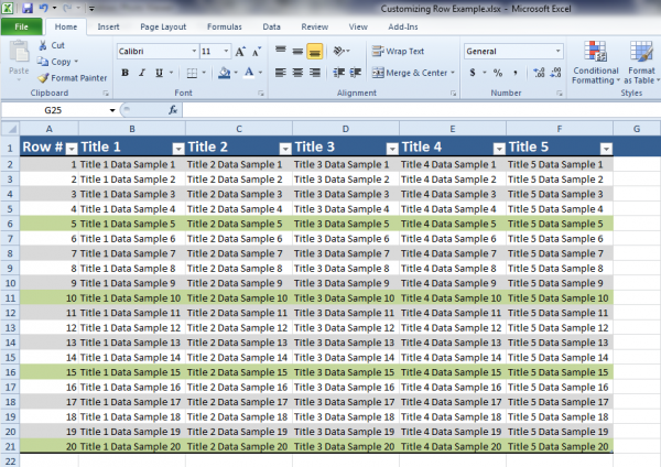
How would I accomplish this with automatic styling?

STEP1:
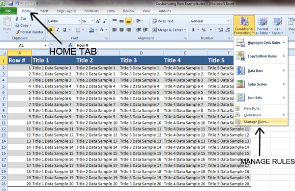
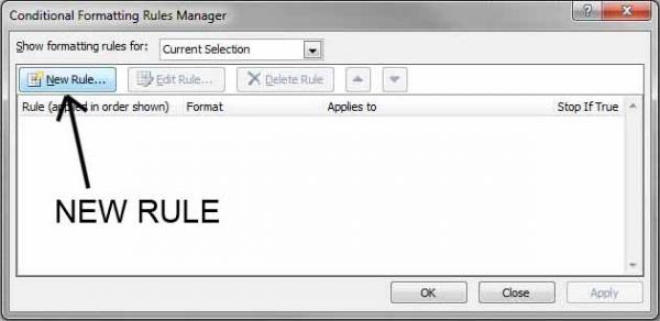
On the Home tab, click Conditional Formatting, then click Manage Rules. Note: You don’t need to highlight the cells before hand to customize your data.

STEP 2:
Click on New Rule

STEP 3:
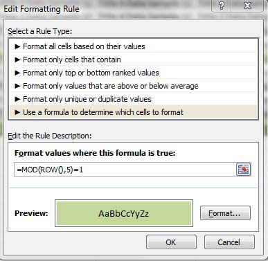
Under New Formatting Rule click Use a formula to determine which cells to format.

At this point, it gets a bit tricky. I want to “modify” every 5th row so I put in

=MOD(ROW(),5)=1

This translate to start on the 1st row and repeat every 5th row. It is very important to kow that the first number MUST be equal to or larger than the second number. Here is the INCORRECT way of doing it: =MOD(ROW(),5)=6, meaning I would start on the 6th row, and repeat every 5 rows. A screenshot of the correct method is shown below.

STEP 4:
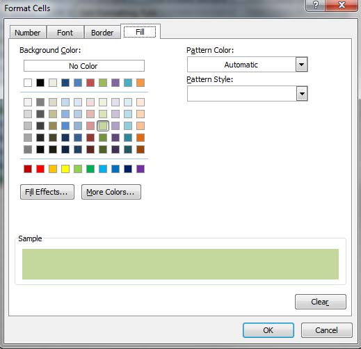
To choose your format, click on FORMAT. From here you can change the font size, add a font style such as adding a bold to your font, add a border, or in my case, go to FILL and select a background.

STEP 5:
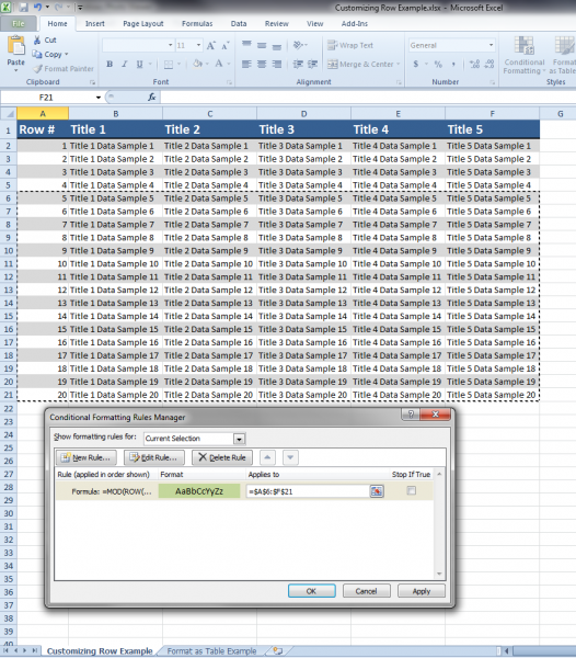
Select the data to apply the rule.

Now remember that my formula was =MOD(ROW(),5)=1, meaning to start on the 1st row and repeat every 5 rows. So for my data I start selecting on the 5th row because my formula considers this my 1st row.

Apply the settings and you get:

Additional information can be found on Microsoft’s blogs.
http://office.microsoft.com/en-us/excel-help/apply-shading-to-alternate-rows-in-a-worksheet-HA010251644.aspx?pid=CH100648351033